|
Size: 10138
Comment:
|
Size: 23078
Comment:
|
| Deletions are marked like this. | Additions are marked like this. |
| Line 2: | Line 2: |
| [[FsTutorial/Diffusion|top]] | [[FsTutorial/TraculaOutputs|previous]] | [[FsTutorial/TraculaGroupAnalysis|next]] = Tract Statistics = This section of the tutorial will teach you to extract Statistical measures along the major White Matter tracts reconstructed by Tracula. There are two types of statistics files that are output for each White Matter Tract * path.overall.txt - This file gives Diffusion measures along the whole WM tract * path.byvoxel.txt - This files gives Diffusion measures for each voxel along the WM tract. To view the statistics files from Tracula for for the subject Diff001 (Left Cortico-Spinal Tract), type the following in the terminal |
[[https://surfer.nmr.mgh.harvard.edu/fswiki/Tutorials|Back to list of all tutorials]] | [[FsTutorial|Back to course page]] | [[FsTutorial/TraculaOutputs|Previous]] = Tract statistics = ||<bgcolor="#CCEEFF">Please bear with us while we update the tutorial data set for the new version of TRACULA. The new tutorial goes beyond what was possible with the tutorial data set that was previously available for download. For now, please ignore any references to the tutorial data and try to follow along using your own data. Thank you for your patience.|| === Remember... === For '''each new''' terminal that you open, you must do: {{{ export SUBJECTS_DIR=$TUTORIAL_DATA/diffusion_tutorial/fs cd $TUTORIAL_DATA/diffusion_tutorial }}} ------- This section of the tutorial will teach you how to extract statistics on anisotropy and diffusivity measures for the white-matter pathways reconstructed by TRACULA. There are two types of statistics files that are created for each white-matter pathway: * '''pathstats.overall.txt''' - This file contains diffusion measures averaged over the whole pathway. * '''pathstats.byvoxel.txt''' - This file contains diffusion measures averaged at consecutive cross-sections of the pathway, resulting in an along-tract profile of each diffusion measure. This type of analysis is referred to as [[https://pubmed.ncbi.nlm.nih.gov/15906294/|pointwise assessment of streamline tractography attributes]] (PASTA). These are plain text files that you can open with a text editor, such as {{{gedit}}} on Linux, or with the command {{{open -e}}} on a Mac. They are saved in the TRACULA output directory of each individual tract. == Anisotropy and diffusivity averaged over an entire pathway == Examine the whole-tract statistics for the left inferior longitudinal fasciculus (ILF) of subject1, by runnning: {{{ cat trc/subject1/dpath/lh.ilf_avg16_syn_bbr/pathstats.overall.txt }}} This file will look like this: {{{ # Title Pathway Statistics # # generating_program /usr/local/freesurfer/7.2.0-beta/bin/dmri_pathstats # cvs_version ayendiki-local # cmdline /usr/local/freesurfer/7.2.0-beta/bin/dmri_pathstats --intrc /space/erebus/1/users/data/trc/subject1/dpath/lh.ilf_avg16_syn_bbr --dtbase /space/erebus/1/users/data/trc/subject1/dmri/dtifit --path lh.ilf --subj subject1 --invox path.ref.txt --out /space/erebus/1/users/data/trc/subject1/dpath/lh.ilf_avg16_syn_bbr/pathstats.overall.txt --outvox /space/erebus/1/users/data/trc/subject1/dpath/lh.ilf_avg16_syn_bbr/pathstats.byvoxel.txt # sysname Linux # hostname compute-0-124.nmr.mgh.harvard.edu # machine x86_64 # user ayendiki # anatomy_type pathway # # subjectname subject # pathwayname lh.ilf # Count 1500 Volume 1996 Len_Min 53 Len_Max 129 Len_Avg 79.9787 Len_Center 89 AD_Avg 0.00120044 AD_Avg_Weight 0.00121209 AD_Avg_Center 0.00123318 RD_Avg 0.000467543 RD_Avg_Weight 0.000458132 RD_Avg_Center 0.000549716 MD_Avg 0.000711842 MD_Avg_Weight 0.000709453 MD_Avg_Center 0.000777538 FA_Avg 0.540167 FA_Avg_Weight 0.553683 FA_Avg_Center 0.477498 }}} This text file contains various diffusion measures, averaged over the entire pathway (in this example, the left ILF). The measures include: * Number of sample paths drawn from the probability distribution of the pathway (Count) * Volume of the probability distribution of the pathway (in voxels) * Maximum, minimum, and average length of the sample paths (in voxels) * Length of the highest-probability (a.k.a. maximum a posteriori) path * Axial diffusivity (average over the entire support of the path distribution, weighted average over the entire support of the path distribution, and average over highest-probability path only) * Radial diffusivity (as above) * Mean diffusivity (as above) * Fractional anisotropy (as above) === Concatenate for group analyses === Measures can be extracted from these files and concatenated across subjects, ''e.g.,'' for group analysis. Specifically, the text files can be converted into a table using the command {{{tractstats2table}}} and then used for doing GLM analyses with [[mri_glmfit]] or any other statistical software (SPSS, Excel, Statview etc.) Before using {{{tractstats2table}}}, you have to create a text file that lists the full path to the {{{pathstats.overall.txt}}} files from all subjects that you want to include in your analysis. For example, if you wanted to analyze whole-tract measures from the left ILF of 3 subjects, you would create a text file that looks like the following: {{{ trc/subject1/dpath/lh.ilf_avg16_syn_bbr/pathstats.overall.txt trc/subject2/dpath/lh.ilf_avg16_syn_bbr/pathstats.overall.txt trc/subject3/dpath/lh.ilf_avg16_syn_bbr/pathstats.overall.txt }}} Create a text file called {{{lh.ilf.list}}} using the command below. Copy and paste the list above into this file, then save the file and exit the editor. {{{ gedit lh.ilf.list & }}} '''ON MACS, RUN:''' {{{ open -e lh.ilf.list & }}} The following command will use this list to create a table with the diffusion measures from all the subjects listed above: {{{ tractstats2table --load-pathstats-from-file lh.ilf.list --overall --tablefile lh.ilf.All.table }}} * The argument to the {{{--load-pathstats-from-file}}} option specifies the text file that contains the list of all the statistics files that will be combined. Take a look at the resulting table file: {{{ gedit lh.ilf.All.table & }}} '''ON MACS, RUN:''' {{{ open -e h.ilf.All.table & }}} Instead of extracting all measures included in the {{{pathstats.overall.txt}}} files, we are usually interested only in a few specific measures. For example, to extract only the average FA for each subject, do the following: {{{ tractstats2table --load-pathstats-from-file $lh.ilf.list --overall --only-measures FA_Avg --tablefile lh.ilf.FA_Avg.table }}} * The argument to the {{{--only-measures}}} option specifies which measure we want to extract from the statistics files. Instead of FA_Avg, this could be the name of any of the measures included in {{{pathstats.overall.txt.}}} '''OPTIONAL:''' You can look at these tables in !OpenOffice (or any other spreadsheet program). For example, to open the file {{{lh.ilf.All.table}}} in !OpenOffice, do the following : {{{ localc lh.ilf.All.table }}} You can then use these stats tables as input to [[mri_glmfit]], to run perform group analysis. == Anisotropy and diffusivity along the trajectory of a pathway == Now examine the along-tract (PASTA) statistics for the left ILF, by running: {{{ cat trc/subject1/dpath/lh.ilf_avg16_syn_bbr/pathstats.byvoxel.txt }}} {{{ # Title Pathway Statistics # # generating_program /usr/local/freesurfer/7.2.0-beta/bin/dmri_pathstats # cvs_version ayendiki-local # cmdline /usr/local/freesurfer/7.2.0-beta/bin/dmri_pathstats --intrc /space/erebus/1/users/data/trc/subject1/dpath/lh.ilf_avg16_syn_bbr --dtbase /space/erebus/1/users/data/trc/subject1/dmri/dtifit --path lh.ilf --subj subject1 --invox path.ref.txt --out /space/erebus/1/users/data/trc/subject1/dpath/lh.ilf_avg16_syn_bbr/pathstats.overall.txt --outvox /space/erebus/1/users/data/trc/subject1/dpath/lh.ilf_avg16_syn_bbr/pathstats.byvoxel.txt # sysname Linux # hostname compute-0-124.nmr.mgh.harvard.edu # machine x86_64 # user ayendiki # anatomy_type pathway # # subjectname subject1 # pathwayname lh.ilf # # pathway start x y z AD RD MD FA AD_Avg RD_Avg MD_Avg FA_Avg 97 78 16 0.000867977 0.000725794 0.000773188 0.108892 0.00107168 0.000599572 0.000756942 0.363722 97 78 16 0.000867977 0.000725794 0.000773188 0.108892 0.00107168 0.000599572 0.000756942 0.363722 97 77 16 0.000832794 0.000712196 0.000752395 0.098711 0.00106892 0.000599915 0.000756251 0.363217 97 77 16 0.000832794 0.000712196 0.000752395 0.098711 0.00106892 0.000599915 0.000756251 0.363217 96 77 17 0.000778157 0.000713259 0.000734892 0.0524794 0.00106822 0.000599456 0.000755712 0.364947 96 76 17 0.000872096 0.000706771 0.000761879 0.136309 0.00106737 0.00059909 0.000755185 0.365999 96 76 17 0.000872096 0.000706771 0.000761879 0.136309 0.00106737 0.00059909 0.000755185 0.365999 96 75 18 0.00106175 0.000671836 0.000801806 0.326543 0.00106621 0.000593117 0.000750814 0.370047 96 74 19 0.00084758 0.000742526 0.000777544 0.146359 0.00107689 0.000564038 0.000734991 0.399445 96 74 19 0.00084758 0.000742526 0.000777544 0.146359 0.00107689 0.000564038 0.000734991 0.399445 96 73 20 0.00105676 0.000582545 0.000740616 0.379989 0.00109462 0.000529155 0.000717645 0.442998 96 73 20 0.00105676 0.000582545 0.000740616 0.379989 0.00109462 0.000529155 0.000717645 0.442998 96 73 21 0.00106829 0.000535296 0.000712959 0.446277 0.00110578 0.000510944 0.000709221 0.466119 96 73 21 0.00106829 0.000535296 0.000712959 0.446277 0.00110578 0.000510944 0.000709221 0.466119 96 72 21 0.00112798 0.000524413 0.000725602 0.490875 0.00109594 0.000500484 0.000698966 0.476156 96 72 22 0.00100371 0.000518413 0.00068018 0.466196 0.00109198 0.000491746 0.000691821 0.484992 96 71 22 0.00110846 0.000516744 0.000713983 0.496827 0.00107691 0.000488262 0.000684476 0.487281 96 70 23 0.000963374 0.000468995 0.000633788 0.515347 0.00103651 0.000500421 0.000679117 0.471307 96 70 24 0.000952905 0.00052878 0.000670155 0.464126 0.00102183 0.000507845 0.000679174 0.463955 96 69 25 0.000941334 0.000510755 0.000654282 0.452879 0.0010153 0.000520488 0.000685426 0.451515 96 69 25 0.000941334 0.000510755 0.000654282 0.452879 0.0010153 0.000520488 0.000685426 0.451515 96 68 25 0.000937902 0.000498823 0.000645183 0.473998 0.0010151 0.000521116 0.000685777 0.45532 96 67 26 0.00114779 0.000422178 0.00066405 0.597208 0.00106285 0.000495767 0.000684795 0.488664 96 67 26 0.00114779 0.000422178 0.00066405 0.597208 0.00106285 0.000495767 0.000684795 0.488664 96 66 27 0.00119928 0.000456432 0.000704049 0.567628 0.00113942 0.000464739 0.000689633 0.535918 96 66 27 0.00119928 0.000456432 0.000704049 0.567628 0.00113942 0.000464739 0.000689633 0.535918 96 65 27 0.00141769 0.000388493 0.000731558 0.691121 0.00118206 0.000446907 0.000691963 0.56636 96 64 28 0.00139466 0.000325184 0.000681676 0.734954 0.00123269 0.000410431 0.000684517 0.612061 96 64 28 0.00139466 0.000325184 0.000681676 0.734954 0.00123269 0.000410431 0.000684517 0.612061 96 63 28 0.00143303 0.000312452 0.000685979 0.752811 0.00126731 0.000393664 0.000684881 0.636549 95 62 29 0.00130884 0.000290893 0.000630209 0.745983 0.00129524 0.000387733 0.000690235 0.648474 94 62 29 0.00164671 0.00076911 0.00106164 0.446289 0.00129674 0.000390088 0.000692304 0.647809 94 61 29 0.00172456 0.000745308 0.00107172 0.485371 0.00127988 0.000398742 0.000692451 0.638261 94 60 30 0.00140745 0.000880179 0.00105594 0.281852 0.00125246 0.000428793 0.00070335 0.606134 94 60 30 0.00140745 0.000880179 0.00105594 0.281852 0.00125246 0.000428793 0.00070335 0.606134 94 59 31 0.00155751 0.000862578 0.00109422 0.356395 0.00121421 0.000460178 0.000711525 0.56957 94 58 32 0.00130825 0.000701944 0.000904047 0.376433 0.00120559 0.000462724 0.00071035 0.562654 94 58 32 0.00130825 0.000701944 0.000904047 0.376433 0.00120559 0.000462724 0.00071035 0.562654 94 57 33 0.00127009 0.000453103 0.000725431 0.580671 0.001259 0.000436023 0.000710351 0.597881 94 56 34 0.00128442 0.000408392 0.0007004 0.624911 0.00131045 0.000409303 0.000709684 0.635395 94 56 34 0.00128442 0.000408392 0.0007004 0.624911 0.00131045 0.000409303 0.000709684 0.635395 94 55 34 0.00129227 0.00046328 0.00073961 0.577816 0.0013183 0.000405609 0.000709842 0.640691 94 54 35 0.0012703 0.000405959 0.000694073 0.624761 0.00132773 0.000405781 0.000713098 0.639696 94 54 36 0.0012825 0.000416241 0.000704992 0.62111 0.00131601 0.00041376 0.000714509 0.62888 94 54 36 0.0012825 0.000416241 0.000704992 0.62111 0.00131601 0.00041376 0.000714509 0.62888 93 53 36 0.00139747 0.000604594 0.000868887 0.488666 0.00130335 0.000422725 0.000716265 0.616271 93 52 36 0.00135543 0.000585794 0.000842337 0.488772 0.0012934 0.000424784 0.000714323 0.612202 93 52 37 0.00123236 0.000470209 0.000724259 0.552723 0.00128567 0.000433751 0.000717722 0.600983 93 51 38 0.00114102 0.000441359 0.00067458 0.550956 0.00128498 0.000448106 0.000727063 0.587959 93 50 38 0.00115213 0.00050062 0.000717791 0.500001 0.00128811 0.00045668 0.00073382 0.580909 93 50 39 0.00106929 0.000415801 0.000633631 0.546817 0.00129122 0.00045262 0.000732149 0.585613 92 49 39 0.00139456 0.000653969 0.000900833 0.448212 0.00129614 0.000456588 0.000736437 0.583877 92 48 39 0.00121658 0.000614545 0.000815223 0.410542 0.00129869 0.00045225 0.000734397 0.588016 92 48 39 0.00121658 0.000614545 0.000815223 0.410542 0.00129869 0.00045225 0.000734397 0.588016 92 47 40 0.00118115 0.000483847 0.000716281 0.521239 0.0013064 0.00044644 0.000733091 0.593569 91 46 41 0.00132381 0.000679848 0.000894501 0.400171 0.00130968 0.000445202 0.000733361 0.593125 91 46 41 0.00132381 0.000679848 0.000894501 0.400171 0.00130968 0.000445202 0.000733361 0.593125 91 45 41 0.00113019 0.000529645 0.000729826 0.454707 0.001325 0.000431276 0.000729183 0.607594 91 44 41 0.00117487 0.000464237 0.000701113 0.530762 0.00134519 0.00041734 0.000726622 0.623841 90 43 41 0.00121382 0.000492301 0.000732807 0.519596 0.00135435 0.00040553 0.000721804 0.635504 90 42 42 0.00141832 0.000419311 0.000752312 0.650028 0.00135835 0.000396281 0.000716967 0.644296 90 41 43 0.00149731 0.000356095 0.0007365 0.72266 0.00135424 0.000393535 0.00071377 0.64191 89 40 43 0.001381 0.000513018 0.000802344 0.564421 0.00132657 0.000407598 0.000713924 0.624407 89 40 43 0.001381 0.000513018 0.000802344 0.564421 0.00132657 0.000407598 0.000713924 0.624407 90 39 43 0.00157585 0.000295255 0.000722119 0.787805 0.00130086 0.000413205 0.00070909 0.613173 89 38 43 0.00138324 0.000383207 0.000716551 0.674917 0.00125725 0.000434189 0.000708544 0.581023 89 38 44 0.00124692 0.000510601 0.000756042 0.514663 0.001253 0.000438098 0.000709733 0.575357 89 37 45 0.00118923 0.00056238 0.000771331 0.44532 0.00122624 0.00044834 0.000707639 0.557656 88 37 45 0.00109356 0.000633894 0.000787115 0.365015 0.00123292 0.000451307 0.000711844 0.55797 88 36 45 0.00103814 0.000676695 0.000797177 0.316449 0.00120901 0.000458568 0.000708718 0.544602 88 35 45 0.00114301 0.000589147 0.000773767 0.391688 0.00118172 0.000467419 0.000705519 0.529077 87 35 45 0.00105685 0.000666853 0.000796853 0.331352 0.00118345 0.000475253 0.000711318 0.523537 87 34 45 0.00125167 0.000637577 0.000842276 0.399288 0.001166 0.000479059 0.000708037 0.516315 87 34 45 0.00125167 0.000637577 0.000842276 0.399288 0.001166 0.000479059 0.000708037 0.516315 87 34 45 0.00125167 0.000637577 0.000842276 0.399288 0.001166 0.000479059 0.000708037 0.516315 86 33 46 0.000997102 0.000709494 0.000805363 0.312391 0.00117978 0.000484607 0.00071633 0.51874 86 33 46 0.000997102 0.000709494 0.000805363 0.312391 0.00117978 0.000484607 0.00071633 0.51874 86 32 46 0.00144502 0.000577058 0.00086638 0.524286 0.00118822 0.000480466 0.000716384 0.525261 86 32 46 0.00144502 0.000577058 0.00086638 0.524286 0.00118822 0.000480466 0.000716384 0.525261 85 31 46 0.00145415 0.000575363 0.000868292 0.528119 0.00121054 0.000477254 0.000721682 0.534651 85 31 46 0.00145415 0.000575363 0.000868292 0.528119 0.00121054 0.000477254 0.000721682 0.534651 85 31 46 0.00145415 0.000575363 0.000868292 0.528119 0.00121054 0.000477254 0.000721682 0.534651 85 30 46 0.00161654 0.000434083 0.000828234 0.688725 0.00121171 0.000469266 0.000716745 0.540934 85 30 46 0.00161654 0.000434083 0.000828234 0.688725 0.00121171 0.000469266 0.000716745 0.540934 85 30 46 0.00161654 0.000434083 0.000828234 0.688725 0.00121171 0.000469266 0.000716745 0.540934 85 29 45 0.00159702 0.000373003 0.00078101 0.732022 0.00120427 0.000464151 0.000710859 0.54041 84 29 45 0.00149992 0.000433867 0.000789218 0.665445 0.0012176 0.000470298 0.000719398 0.53854 84 29 45 0.00149992 0.000433867 0.000789218 0.665445 0.0012176 0.000470298 0.000719398 0.53854 84 29 45 0.00149992 0.000433867 0.000789218 0.665445 0.0012176 0.000470298 0.000719398 0.53854 # pathway end }}} This text file contains various diffusion measures, one row for each position along the trajectory of the path. The first three entries in each row are the x, y, z coordinates in native diffusion space. The next four entries are the axial diffusivity, radial diffusivity, mean diffusivity, and fractional anisotropy at that position on the maximum a posteriori path. The last four entries are the axial diffusivity, radial diffusivity, mean diffusivity, and fractional anisotropy at the same position, averaged over all sampled paths. Points are ordered according to the following convention (see also [[https://dmri.mgh.harvard.edu/tract-atlas/|along-tract plots]]): * For pathways with a right-left orientation: * If the pathway is inter-hemispheric: From right to left * If the pathway is intra-hemispheric: From medial to lateral * For pathways with an anterior-posterior orientation: From anterior to posterior * For pathways with a superior-inferior orientation: From superior to inferior === Converting pathstats.byvoxel.txt files to a table for group analyses === You can combine the '''pathstats.byvoxel.txt''' files from multiple subjects, to use as input for along-tract group analysis, by running the following: {{{ trac-all -stat -c $TUTORIAL_DATA/diffusion_tutorial/dmrirc.tutorial }}} This will create a directory named {{{stats}}} under the main TRACULA output directory and save one table per tract per diffusion measure. In these tables, each row is a different position along the trajectory of the tract and each column is a different subject. To examine the table of average FA along the left ILF, do the following: {{{ gedit trc/stats/lh.ilf.avg16_syn_bbr.FA_Avg.txt & }}} '''ON MACS, RUN:''' {{{ open -e trc/stats/lh.ilf.avg16_syn_bbr.FA_Avg.txt & }}} The contents of this file will look like this: {{{ elmo.2005 elmo.2008 elmo.2012 NaN NaN 0.378069 NaN NaN 0.378492 0.41336 NaN 0.388788 0.429444 0.377014 0.4164 0.444207 0.392511 0.438363 0.452544 0.394491 0.445661 0.449954 0.388662 0.435143 0.447727 0.407221 0.426532 0.432298 0.428718 0.421008 0.419581 0.425808 0.403944 0.473702 0.40381 0.371384 0.494473 0.387531 0.353198 0.4767 0.414657 0.366791 0.506063 0.453886 0.412596 0.583493 0.519466 0.483278 0.624087 0.57846 0.549247 0.647596 0.600432 0.569196 ... }}} The first row tells you the subject names for the corresponding columns of FA values. You can use these stats tables to run a group analysis on the tracts. '''Note:''' In addition to the above tables, the {{{stats}}} directory will also contain a log file for each pathway. You can examine the log file, which contains the full output of the {{{trac-all -stat}}} command, to see if any pathways were flagged as outliers. If this happens, there will be a line in the log file with {{{"Found outlier path:"}}} and the name of the subject. These are paths that were found to differ excessively from those of the other subjects. You can check this information to find out if the reconstruction of this tract failed for any subjects. For example, you can examine the log file for the left ILF by doing: {{{ gedit trc/stats/lh.ilf.avg16_syn_bbr.log & }}} '''ON MACS, RUN:''' {{{ open -e trc/stats/lh.ilf.avg16_syn_bbr.log & }}} === Visualizing results from statistical analyses along each pathway === By default, TRACULA uses the mean of its manually annotated training streamlines to determine the positions along each of the 42 pathways where diffusion measures will be projected. These mean streamlines are saved in template space (the template that is the target of the inter-subject registration) and mapped to each individual subject after the individual subjects pathways are reconstructed, to extract the along-tract measures. Note that these mean paths are only used to determine how each pathway will sliced up into into cross-sections where along-tract measures will be averaged, and to ensure an equal number of cross-sections for all subjects. To view all 42 mean paths in template space, run the following: {{{ freeview -v $FREESURFER_HOME/trctrain/hcp/MGH35_HCP_FA_template.nii.gz \ -t $FREESURFER_HOME/trctrain/hcp/syn/*.mean.trk }}} You should see something like this in the 3D view: {{attachment:path.waypts.jpg}} {{{#!wiki caution The following information is based on hypothetical statistical data. The text file of p-values is not available so do not expect your end result to look identical to this image. }}} Let's say that you have performed a statistical analysis on your subjects in your statistical software of choice. If you save the p-values corresponding to each position along a tract to a simple text file, you can now display these p-values as a heat map on the corresponding mean path. (It is assumed that the number of p-values in your text file is equal to the number of points on the mean path, which is the same as the number of rows of values in the group tables produced by {{{trac-all -stat.}}} If not, display may be problematic.) To display the p-values from your hypothetical analysis on one of the mean paths, do the following: * Select the mean path of your choice on the panel in the top left of the freeview window. On the left menu, click on {{{Show spline}}}. * From the {{{Spline color}}} menu, choose {{{Heatscale}}}. * From the {{{Scalar map}}} menu, choose {{{Load...}}} and select the text file that contains the p-values from your statistical analysis. * To hide the waypoints, which show up as small spheres, increase the {{{Spline radius}}} so that it is greater than the {{{Radius}}} of the waypoints. (In the example below, we have set the {{{Spline radius}}} to 2, while the {{{Radius}}} of the waypoints is 1.) * Set the {{{Min,}}} {{{Mid,}}} and {{{Max}}} of the heatscale to threshold the p-values as you wish. You can do this for as many of the tracts as you have performed statistical analyses on. The end result will look something like this in the 3D view: {{attachment:path.waypts.p.jpg}} -------- = Summary = By the end of this page, you should know how to: * Extract statistics (anisotropy and diffusivity measures), either averaged over an entire white-matter pathway, or as a function of position along the trajectory of the pathway * Combine statistics into tables for group analysis * Perform whole-tract and along-tract statistical analysis * Visualize the outputs of along-tract statistical analysis in freeview |
| Line 12: | Line 347: |
| {{{ cd $TUTORIAL_DATA/diffusion_tutorial/Diff001/dpath/5cpts/priorcvs/seg14/initmni/regbbr/lh.cst_AS_avg23_cvs_bbr/ less path.overall.txt less path.byvoxel.txt }}} ---- == path.overall.txt == This text file gives various diffusion measures about the specific white matter tract along its complete path. Some of the measures include: * Count of the # of Fibers in the WM tract * Tract Volume * Maximum, Minimum and Average length of fibers * Length of the center fiber * Axial Diffusivity (both average and along the center) * Radial Diffusivity (both average and along the center) * Mean Diffusivity (both average and along the center) * Fractional Anisotropy (both average and along the center) ---- {{{ # Title Pathway Statistics # # generating_program $FREESURFER_HOME/bin/dmri_pathstats # cvs_version # cmdline $FREESURFER_HOME/bin/dmri_pathstats --intrc $TUTORIAL_DATA/diffusion_tutorial/Diff001/dpath/5cpts/priorcvs/seg14/initmni/regbbr/lh.cst_AS_avg23_cvs_bbr --dtbase $TUTORIAL_DATA/diffusion_tutorial/Diff001/dmri/dtifit --path lh.cst --subj Diff001 --out $TUTORIAL_DATA/diffusion_tutorial/Diff001/dpath/5cpts/priorcvs/seg14/initmni/regbbr/lh.cst_AS_avg23_cvs_bbr/pathstats.overall.txt --outvox $TUTORIAL_DATA/diffusion_tutorial/Diff001/dpath/5cpts/priorcvs/seg14/initmni/regbbr/lh.cst_AS_avg23_cvs_bbr/pathstats.byvoxel.txt # sysname Linux # hostname compute-0-1.local # machine x86_64 # user rspriti # anatomy_type pathway # # subjectname Diff001 # pathwayname lh.cst # Count 100 Volume 235 Len_Min 45 Len_Max 69 Len_Avg 55.3 Len_Center 53 AD_Avg 0.00108402 AD_Avg_Weight 0.00107521 AD_Avg_Center 0.00107062 RD_Avg 0.00046958 RD_Avg_Weight 0.000476065 RD_Avg_Center 0.000507009 MD_Avg 0.000674393 MD_Avg_Weight 0.000675781 MD_Avg_Center 0.000694881 FA_Avg 0.50122 FA_Avg_Weight 0.48976 FA_Avg_Center 0.456292 }}} ---- == path.byvoxel.txt == This text file gives us various diffusion measures in each voxel along the WM tract ---- {{{ # Title Pathway Statistics # # generating_program $FREESURFER_HOME/dmri_pathstats # cvs_version # cmdline $FREESURFER_HOME/dmri_pathstats --intrc $TUTORIAL_DATA/diffusion_tutorial/Diff001/dpath/5cpts/priorcvs/seg14/initmni/regbbr/lh.cst_AS_avg23_cvs_bbr --dtbase $TUTORIAL_DATA/diffusion_tutorial/Diff001/dmri/dtifit --path lh.cst --subj Diff001 --out $TUTORIAL_DATA/diffusion_tutorial/Diff001/dpath/5cpts/priorcvs/seg14/initmni/regbbr/lh.cst_AS_avg23_cvs_bbr/pathstats.overall.txt --outvox $TUTORIAL_DATA/diffusion_tutorial/Diff001/dpath/5cpts/priorcvs/seg14/initmni/regbbr/lh.cst_AS_avg23_cvs_bbr/pathstats.byvoxel.txt # sysname Linux # hostname compute-0-1.local # machine x86_64 # user rspriti # anatomy_type pathway # # subjectname Diff001 # pathwayname lh.cst # # pathway start x y z AD RD MD FA 62 63 10 0.000637887 0.000476948 0.000530594 0.178865 62 63 11 0.0006074 0.000433505 0.00049147 0.22773 63 63 12 0.000846852 0.000610935 0.000689574 0.251636 63 64 13 0.00123916 0.00105259 0.00111478 0.107897 63 64 14 0.000936783 0.000621757 0.000726766 0.264886 64 64 15 0.000869413 0.000500918 0.00062375 0.348479 64 64 16 0.000742746 0.000432898 0.000536181 0.357518 65 64 16 0.000729103 0.000361411 0.000483975 0.42985 66 65 17 0.000645165 0.000105291 0.000285249 0.86012 67 65 18 0.00115478 0.000351219 0.000619072 0.647404 68 66 19 0.00142292 0.000690686 0.000934763 0.432432 69 66 20 0.00166259 0.000912869 0.00116278 0.363279 69 66 21 0.00145087 0.000448438 0.000782583 0.639517 70 66 22 0.00124617 0.000204701 0.000551856 0.816332 70 66 23 0.00138642 0.000415134 0.000738896 0.650657 71 66 23 0.00136252 0.000330065 0.000674217 0.721118 71 66 24 0.00134187 0.000385197 0.000704089 0.678151 71 66 25 0.00108983 0.000289931 0.000556565 0.729769 72 66 26 0.00106165 0.000357968 0.000592529 0.650427 72 66 27 0.00117242 0.000398032 0.00065616 0.619191 73 65 28 0.00130606 0.000441963 0.000729994 0.61662 73 65 29 0.00132239 0.00034928 0.000673651 0.701421 74 65 30 0.00133145 0.000391918 0.000705096 0.652609 74 65 31 0.00130265 0.000371743 0.000682045 0.665608 74 65 32 0.00126357 0.000429947 0.000707822 0.596254 75 65 33 0.00126146 0.000533254 0.000775991 0.499365 75 64 34 0.00117235 0.000465188 0.00070091 0.536046 75 64 35 0.00111144 0.000424831 0.000653701 0.560041 76 64 36 0.00128036 0.000299521 0.000626469 0.731721 76 64 37 0.00119495 0.000322181 0.000613105 0.688909 76 64 38 0.00105691 0.000334124 0.000575053 0.64994 76 63 39 0.00106784 0.000449252 0.000655449 0.514129 76 63 40 0.00113234 0.000537139 0.000735539 0.463226 76 63 41 0.000990485 0.000493054 0.000658864 0.446701 76 63 42 0.000798778 0.000477672 0.000584708 0.336071 76 62 43 0.000870652 0.000483175 0.000612334 0.362795 75 62 44 0.000878542 0.000493417 0.000621792 0.376378 75 62 45 0.000897465 0.000514559 0.000642194 0.348244 75 61 46 0.000882752 0.000537658 0.000652689 0.310019 74 61 47 0.00100985 0.00048457 0.000659663 0.436199 74 61 48 0.00104135 0.000461786 0.000654973 0.482846 74 60 49 0.000957188 0.000488566 0.000644774 0.472547 73 60 50 0.00100422 0.00055232 0.000702954 0.378698 73 60 51 0.000938077 0.000492242 0.000640854 0.429111 72 59 52 0.00104503 0.000475882 0.000665599 0.474443 72 59 53 0.00091483 0.00047261 0.000620017 0.409087 72 59 54 0.000792557 0.000632776 0.000686036 0.174565 71 59 55 0.000961412 0.000680667 0.000774249 0.243739 71 58 56 0.001061 0.000895478 0.000950651 0.133396 70 58 57 0.000862592 0.000663684 0.000729986 0.162365 70 58 58 0.00119199 0.00103056 0.00108437 0.086213 69 57 59 0.00120589 0.000980809 0.00105584 0.127098 69 57 60 0.00102806 0.000829161 0.000895461 0.141788 # pathway end }}} ---- These two files can be used to extract measures that can be further used group analysis. This can also be converted into a table using tractstats2table for doing GLM analyses using mri_glmfit or any other statistical software (SPSS, Excel, Statview etc) === path.overall.txt to Table Conversion === To extract all diffusion measures into a table do the following: ---- {{{ tractstats2table --inputs $TUTORIAL_DATA/diffusion_tutorial/Diff001/dpath/5cpts/priorcvs/seg14/initmni/regbbr/lh.cst_AS_avg23_cvs_bbr/pathstats.overall.txt --overall --tablefile Diff001_LH.CST.All.Priorcvs.table }}} ---- Instead of extracting all the measures from path.overall.txt, we can get specific measures that can be used for group analysis.For example, to extract only the Average Fractional Anisotropy along Left Cortico-spinal tract, do the following: ---- {{{ tractstats2table --inputs $TUTORIAL_DATA/diffusion_tutorial/Diff001/dpath/5cpts/priorcvs/seg14/initmni/regbbr/lh.cst_AS_avg23_cvs_bbr/pathstats.overall.txt --overall --only-measures FA_Avg --tablefile Diff001_LH.CST.FA.Priorcvs.table }}} ---- For a group analysis that has multiple subjects, '''tractstats2table''' can be used to combine all the subjects' diffusion measures from path.overall.txt into a single table that can be used for analysis with mri_glmfit or any other statistics software An easy way to do this is to create a text file that contains the names of the subjects and paths to their path.overall.txt files. An example is given below: ---- {{{ $TUTORIAL_DATA/Diff001/dpath/priorcvs/regbbr/lh.cst_AS_avg23_cvs_bbr/pathstats.overall.txt $TUTORIAL_DATA/Diff002/dpath/priorcvs/regbbr/lh.cst_AS_avg23_cvs_bbr/pathstats.overall.txt $TUTORIAL_DATA/Diff003/dpath/priorcvs/regbbr/lh.cst_AS_avg23_cvs_bbr/pathstats.overall.txt $TUTORIAL_DATA/Diff004/dpath/priorcvs/regbbr/lh.cst_AS_avg23_cvs_bbr/pathstats.overall.txt $TUTORIAL_DATA/Diff005/dpath/priorcvs/regbbr/lh.cst_AS_avg23_cvs_bbr/pathstats.overall.txt $TUTORIAL_DATA/Diff006/dpath/priorcvs/regbbr/lh.cst_AS_avg23_cvs_bbr/pathstats.overall.txt $TUTORIAL_DATA/Diff007/dpath/priorcvs/regbbr/lh.cst_AS_avg23_cvs_bbr/pathstats.overall.txt $TUTORIAL_DATA/Diff008/dpath/priorcvs/regbbr/lh.cst_AS_avg23_cvs_bbr/pathstats.overall.txt $TUTORIAL_DATA/Diff009/dpath/priorcvs/regbbr/lh.cst_AS_avg23_cvs_bbr/pathstats.overall.txt $TUTORIAL_DATA/Diff010/dpath/priorcvs/regbbr/lh.cst_AS_avg23_cvs_bbr/pathstats.overall.txt }}} ---- Once this is created and saved as lh_cst_priorcvs_overall_pathstats, it can be passed as a parameter in tractstats2table command. The following command will create a table with all the subjects specified in the lh_cst_priorcvs_overall_pathstats file and all the diffusion measures from '''path.overall.txt''' for each subject. ---- {{{ tractstats2table --load-pathstats-from-file $TUTORIAL_DATA/diffusion_tutorial/TraculaGLM/LesionStudy/lh_cst_priorcvs_overall_pathstats --overall --tablefile LH.CST.All.Priorcvs.table }}} ---- To extract only specific measures like FA_Avg, do the following: ---- {{{ tractstats2table --load-pathstats-from-file $TUTORIAL_DATA/diffusion_tutorial/TraculaGLM/LesionStudy/lh_cst_priorcvs_overall_pathstats --overall --only-measures FA_Avg --tablefile LH.CST.FA.Priorcvs.table }}} ---- You can look at these tables in OpenOffice's spreadsheet program. For example, to open the table '''LH.CST.All.Priorcvs.table''' in a spreadsheet, do the following: ---- {{{ oocalc $TUTORIAL_DATA/diffusion_tutorial/TraculaGLM/LesionStudy/LH.CST.All.Priorcvs.table (Not sure if this will be the final directory...things may have moved around by weekend) }}} ---- |
== Quiz == You can test your knowledge of this tutorial by [[https://forms.gle/ThENqfuVoVtnm1aT9|clicking here]] for a quiz! ----- [[https://surfer.nmr.mgh.harvard.edu/fswiki/Tutorials|Back to list of all tutorials]] | [[FsTutorial|Back to course page]] | [[FsTutorial/TraculaOutputs|Previous]] |
Back to list of all tutorials | Back to course page | Previous
Tract statistics
Please bear with us while we update the tutorial data set for the new version of TRACULA. The new tutorial goes beyond what was possible with the tutorial data set that was previously available for download. For now, please ignore any references to the tutorial data and try to follow along using your own data. Thank you for your patience. |
Remember...
For each new terminal that you open, you must do:
export SUBJECTS_DIR=$TUTORIAL_DATA/diffusion_tutorial/fs
cd $TUTORIAL_DATA/diffusion_tutorial
This section of the tutorial will teach you how to extract statistics on anisotropy and diffusivity measures for the white-matter pathways reconstructed by TRACULA. There are two types of statistics files that are created for each white-matter pathway:
pathstats.overall.txt - This file contains diffusion measures averaged over the whole pathway.
pathstats.byvoxel.txt - This file contains diffusion measures averaged at consecutive cross-sections of the pathway, resulting in an along-tract profile of each diffusion measure. This type of analysis is referred to as pointwise assessment of streamline tractography attributes (PASTA).
These are plain text files that you can open with a text editor, such as gedit on Linux, or with the command open -e on a Mac. They are saved in the TRACULA output directory of each individual tract.
Anisotropy and diffusivity averaged over an entire pathway
Examine the whole-tract statistics for the left inferior longitudinal fasciculus (ILF) of subject1, by runnning:
cat trc/subject1/dpath/lh.ilf_avg16_syn_bbr/pathstats.overall.txt
This file will look like this:
# Title Pathway Statistics
#
# generating_program /usr/local/freesurfer/7.2.0-beta/bin/dmri_pathstats
# cvs_version ayendiki-local
# cmdline /usr/local/freesurfer/7.2.0-beta/bin/dmri_pathstats --intrc /space/erebus/1/users/data/trc/subject1/dpath/lh.ilf_avg16_syn_bbr --dtbase /space/erebus/1/users/data/trc/subject1/dmri/dtifit --path lh.ilf --subj subject1 --invox path.ref.txt --out /space/erebus/1/users/data/trc/subject1/dpath/lh.ilf_avg16_syn_bbr/pathstats.overall.txt --outvox /space/erebus/1/users/data/trc/subject1/dpath/lh.ilf_avg16_syn_bbr/pathstats.byvoxel.txt
# sysname Linux
# hostname compute-0-124.nmr.mgh.harvard.edu
# machine x86_64
# user ayendiki
# anatomy_type pathway
#
# subjectname subject
# pathwayname lh.ilf
#
Count 1500
Volume 1996
Len_Min 53
Len_Max 129
Len_Avg 79.9787
Len_Center 89
AD_Avg 0.00120044
AD_Avg_Weight 0.00121209
AD_Avg_Center 0.00123318
RD_Avg 0.000467543
RD_Avg_Weight 0.000458132
RD_Avg_Center 0.000549716
MD_Avg 0.000711842
MD_Avg_Weight 0.000709453
MD_Avg_Center 0.000777538
FA_Avg 0.540167
FA_Avg_Weight 0.553683
FA_Avg_Center 0.477498
This text file contains various diffusion measures, averaged over the entire pathway (in this example, the left ILF). The measures include:
- Number of sample paths drawn from the probability distribution of the pathway (Count)
- Volume of the probability distribution of the pathway (in voxels)
- Maximum, minimum, and average length of the sample paths (in voxels)
- Length of the highest-probability (a.k.a. maximum a posteriori) path
- Axial diffusivity (average over the entire support of the path distribution, weighted average over the entire support of the path distribution, and average over highest-probability path only)
- Radial diffusivity (as above)
- Mean diffusivity (as above)
- Fractional anisotropy (as above)
Concatenate for group analyses
Measures can be extracted from these files and concatenated across subjects, e.g., for group analysis. Specifically, the text files can be converted into a table using the command tractstats2table and then used for doing GLM analyses with mri_glmfit or any other statistical software (SPSS, Excel, Statview etc.)
Before using tractstats2table, you have to create a text file that lists the full path to the pathstats.overall.txt files from all subjects that you want to include in your analysis. For example, if you wanted to analyze whole-tract measures from the left ILF of 3 subjects, you would create a text file that looks like the following:
trc/subject1/dpath/lh.ilf_avg16_syn_bbr/pathstats.overall.txt
trc/subject2/dpath/lh.ilf_avg16_syn_bbr/pathstats.overall.txt
trc/subject3/dpath/lh.ilf_avg16_syn_bbr/pathstats.overall.txt
Create a text file called lh.ilf.list using the command below. Copy and paste the list above into this file, then save the file and exit the editor.
gedit lh.ilf.list &
ON MACS, RUN:
open -e lh.ilf.list &
The following command will use this list to create a table with the diffusion measures from all the subjects listed above:
tractstats2table --load-pathstats-from-file lh.ilf.list --overall --tablefile lh.ilf.All.table
The argument to the --load-pathstats-from-file option specifies the text file that contains the list of all the statistics files that will be combined.
Take a look at the resulting table file:
gedit lh.ilf.All.table &
ON MACS, RUN:
open -e h.ilf.All.table &
Instead of extracting all measures included in the pathstats.overall.txt files, we are usually interested only in a few specific measures. For example, to extract only the average FA for each subject, do the following:
tractstats2table --load-pathstats-from-file $lh.ilf.list --overall --only-measures FA_Avg --tablefile lh.ilf.FA_Avg.table
The argument to the --only-measures option specifies which measure we want to extract from the statistics files. Instead of FA_Avg, this could be the name of any of the measures included in pathstats.overall.txt.
OPTIONAL: You can look at these tables in OpenOffice (or any other spreadsheet program). For example, to open the file lh.ilf.All.table in OpenOffice, do the following :
localc lh.ilf.All.table
You can then use these stats tables as input to mri_glmfit, to run perform group analysis.
Anisotropy and diffusivity along the trajectory of a pathway
Now examine the along-tract (PASTA) statistics for the left ILF, by running:
cat trc/subject1/dpath/lh.ilf_avg16_syn_bbr/pathstats.byvoxel.txt
# Title Pathway Statistics
#
# generating_program /usr/local/freesurfer/7.2.0-beta/bin/dmri_pathstats
# cvs_version ayendiki-local
# cmdline /usr/local/freesurfer/7.2.0-beta/bin/dmri_pathstats --intrc /space/erebus/1/users/data/trc/subject1/dpath/lh.ilf_avg16_syn_bbr --dtbase /space/erebus/1/users/data/trc/subject1/dmri/dtifit --path lh.ilf --subj subject1 --invox path.ref.txt --out /space/erebus/1/users/data/trc/subject1/dpath/lh.ilf_avg16_syn_bbr/pathstats.overall.txt --outvox /space/erebus/1/users/data/trc/subject1/dpath/lh.ilf_avg16_syn_bbr/pathstats.byvoxel.txt
# sysname Linux
# hostname compute-0-124.nmr.mgh.harvard.edu
# machine x86_64
# user ayendiki
# anatomy_type pathway
#
# subjectname subject1
# pathwayname lh.ilf
#
# pathway start
x y z AD RD MD FA AD_Avg RD_Avg MD_Avg FA_Avg
97 78 16 0.000867977 0.000725794 0.000773188 0.108892 0.00107168 0.000599572 0.000756942 0.363722
97 78 16 0.000867977 0.000725794 0.000773188 0.108892 0.00107168 0.000599572 0.000756942 0.363722
97 77 16 0.000832794 0.000712196 0.000752395 0.098711 0.00106892 0.000599915 0.000756251 0.363217
97 77 16 0.000832794 0.000712196 0.000752395 0.098711 0.00106892 0.000599915 0.000756251 0.363217
96 77 17 0.000778157 0.000713259 0.000734892 0.0524794 0.00106822 0.000599456 0.000755712 0.364947
96 76 17 0.000872096 0.000706771 0.000761879 0.136309 0.00106737 0.00059909 0.000755185 0.365999
96 76 17 0.000872096 0.000706771 0.000761879 0.136309 0.00106737 0.00059909 0.000755185 0.365999
96 75 18 0.00106175 0.000671836 0.000801806 0.326543 0.00106621 0.000593117 0.000750814 0.370047
96 74 19 0.00084758 0.000742526 0.000777544 0.146359 0.00107689 0.000564038 0.000734991 0.399445
96 74 19 0.00084758 0.000742526 0.000777544 0.146359 0.00107689 0.000564038 0.000734991 0.399445
96 73 20 0.00105676 0.000582545 0.000740616 0.379989 0.00109462 0.000529155 0.000717645 0.442998
96 73 20 0.00105676 0.000582545 0.000740616 0.379989 0.00109462 0.000529155 0.000717645 0.442998
96 73 21 0.00106829 0.000535296 0.000712959 0.446277 0.00110578 0.000510944 0.000709221 0.466119
96 73 21 0.00106829 0.000535296 0.000712959 0.446277 0.00110578 0.000510944 0.000709221 0.466119
96 72 21 0.00112798 0.000524413 0.000725602 0.490875 0.00109594 0.000500484 0.000698966 0.476156
96 72 22 0.00100371 0.000518413 0.00068018 0.466196 0.00109198 0.000491746 0.000691821 0.484992
96 71 22 0.00110846 0.000516744 0.000713983 0.496827 0.00107691 0.000488262 0.000684476 0.487281
96 70 23 0.000963374 0.000468995 0.000633788 0.515347 0.00103651 0.000500421 0.000679117 0.471307
96 70 24 0.000952905 0.00052878 0.000670155 0.464126 0.00102183 0.000507845 0.000679174 0.463955
96 69 25 0.000941334 0.000510755 0.000654282 0.452879 0.0010153 0.000520488 0.000685426 0.451515
96 69 25 0.000941334 0.000510755 0.000654282 0.452879 0.0010153 0.000520488 0.000685426 0.451515
96 68 25 0.000937902 0.000498823 0.000645183 0.473998 0.0010151 0.000521116 0.000685777 0.45532
96 67 26 0.00114779 0.000422178 0.00066405 0.597208 0.00106285 0.000495767 0.000684795 0.488664
96 67 26 0.00114779 0.000422178 0.00066405 0.597208 0.00106285 0.000495767 0.000684795 0.488664
96 66 27 0.00119928 0.000456432 0.000704049 0.567628 0.00113942 0.000464739 0.000689633 0.535918
96 66 27 0.00119928 0.000456432 0.000704049 0.567628 0.00113942 0.000464739 0.000689633 0.535918
96 65 27 0.00141769 0.000388493 0.000731558 0.691121 0.00118206 0.000446907 0.000691963 0.56636
96 64 28 0.00139466 0.000325184 0.000681676 0.734954 0.00123269 0.000410431 0.000684517 0.612061
96 64 28 0.00139466 0.000325184 0.000681676 0.734954 0.00123269 0.000410431 0.000684517 0.612061
96 63 28 0.00143303 0.000312452 0.000685979 0.752811 0.00126731 0.000393664 0.000684881 0.636549
95 62 29 0.00130884 0.000290893 0.000630209 0.745983 0.00129524 0.000387733 0.000690235 0.648474
94 62 29 0.00164671 0.00076911 0.00106164 0.446289 0.00129674 0.000390088 0.000692304 0.647809
94 61 29 0.00172456 0.000745308 0.00107172 0.485371 0.00127988 0.000398742 0.000692451 0.638261
94 60 30 0.00140745 0.000880179 0.00105594 0.281852 0.00125246 0.000428793 0.00070335 0.606134
94 60 30 0.00140745 0.000880179 0.00105594 0.281852 0.00125246 0.000428793 0.00070335 0.606134
94 59 31 0.00155751 0.000862578 0.00109422 0.356395 0.00121421 0.000460178 0.000711525 0.56957
94 58 32 0.00130825 0.000701944 0.000904047 0.376433 0.00120559 0.000462724 0.00071035 0.562654
94 58 32 0.00130825 0.000701944 0.000904047 0.376433 0.00120559 0.000462724 0.00071035 0.562654
94 57 33 0.00127009 0.000453103 0.000725431 0.580671 0.001259 0.000436023 0.000710351 0.597881
94 56 34 0.00128442 0.000408392 0.0007004 0.624911 0.00131045 0.000409303 0.000709684 0.635395
94 56 34 0.00128442 0.000408392 0.0007004 0.624911 0.00131045 0.000409303 0.000709684 0.635395
94 55 34 0.00129227 0.00046328 0.00073961 0.577816 0.0013183 0.000405609 0.000709842 0.640691
94 54 35 0.0012703 0.000405959 0.000694073 0.624761 0.00132773 0.000405781 0.000713098 0.639696
94 54 36 0.0012825 0.000416241 0.000704992 0.62111 0.00131601 0.00041376 0.000714509 0.62888
94 54 36 0.0012825 0.000416241 0.000704992 0.62111 0.00131601 0.00041376 0.000714509 0.62888
93 53 36 0.00139747 0.000604594 0.000868887 0.488666 0.00130335 0.000422725 0.000716265 0.616271
93 52 36 0.00135543 0.000585794 0.000842337 0.488772 0.0012934 0.000424784 0.000714323 0.612202
93 52 37 0.00123236 0.000470209 0.000724259 0.552723 0.00128567 0.000433751 0.000717722 0.600983
93 51 38 0.00114102 0.000441359 0.00067458 0.550956 0.00128498 0.000448106 0.000727063 0.587959
93 50 38 0.00115213 0.00050062 0.000717791 0.500001 0.00128811 0.00045668 0.00073382 0.580909
93 50 39 0.00106929 0.000415801 0.000633631 0.546817 0.00129122 0.00045262 0.000732149 0.585613
92 49 39 0.00139456 0.000653969 0.000900833 0.448212 0.00129614 0.000456588 0.000736437 0.583877
92 48 39 0.00121658 0.000614545 0.000815223 0.410542 0.00129869 0.00045225 0.000734397 0.588016
92 48 39 0.00121658 0.000614545 0.000815223 0.410542 0.00129869 0.00045225 0.000734397 0.588016
92 47 40 0.00118115 0.000483847 0.000716281 0.521239 0.0013064 0.00044644 0.000733091 0.593569
91 46 41 0.00132381 0.000679848 0.000894501 0.400171 0.00130968 0.000445202 0.000733361 0.593125
91 46 41 0.00132381 0.000679848 0.000894501 0.400171 0.00130968 0.000445202 0.000733361 0.593125
91 45 41 0.00113019 0.000529645 0.000729826 0.454707 0.001325 0.000431276 0.000729183 0.607594
91 44 41 0.00117487 0.000464237 0.000701113 0.530762 0.00134519 0.00041734 0.000726622 0.623841
90 43 41 0.00121382 0.000492301 0.000732807 0.519596 0.00135435 0.00040553 0.000721804 0.635504
90 42 42 0.00141832 0.000419311 0.000752312 0.650028 0.00135835 0.000396281 0.000716967 0.644296
90 41 43 0.00149731 0.000356095 0.0007365 0.72266 0.00135424 0.000393535 0.00071377 0.64191
89 40 43 0.001381 0.000513018 0.000802344 0.564421 0.00132657 0.000407598 0.000713924 0.624407
89 40 43 0.001381 0.000513018 0.000802344 0.564421 0.00132657 0.000407598 0.000713924 0.624407
90 39 43 0.00157585 0.000295255 0.000722119 0.787805 0.00130086 0.000413205 0.00070909 0.613173
89 38 43 0.00138324 0.000383207 0.000716551 0.674917 0.00125725 0.000434189 0.000708544 0.581023
89 38 44 0.00124692 0.000510601 0.000756042 0.514663 0.001253 0.000438098 0.000709733 0.575357
89 37 45 0.00118923 0.00056238 0.000771331 0.44532 0.00122624 0.00044834 0.000707639 0.557656
88 37 45 0.00109356 0.000633894 0.000787115 0.365015 0.00123292 0.000451307 0.000711844 0.55797
88 36 45 0.00103814 0.000676695 0.000797177 0.316449 0.00120901 0.000458568 0.000708718 0.544602
88 35 45 0.00114301 0.000589147 0.000773767 0.391688 0.00118172 0.000467419 0.000705519 0.529077
87 35 45 0.00105685 0.000666853 0.000796853 0.331352 0.00118345 0.000475253 0.000711318 0.523537
87 34 45 0.00125167 0.000637577 0.000842276 0.399288 0.001166 0.000479059 0.000708037 0.516315
87 34 45 0.00125167 0.000637577 0.000842276 0.399288 0.001166 0.000479059 0.000708037 0.516315
87 34 45 0.00125167 0.000637577 0.000842276 0.399288 0.001166 0.000479059 0.000708037 0.516315
86 33 46 0.000997102 0.000709494 0.000805363 0.312391 0.00117978 0.000484607 0.00071633 0.51874
86 33 46 0.000997102 0.000709494 0.000805363 0.312391 0.00117978 0.000484607 0.00071633 0.51874
86 32 46 0.00144502 0.000577058 0.00086638 0.524286 0.00118822 0.000480466 0.000716384 0.525261
86 32 46 0.00144502 0.000577058 0.00086638 0.524286 0.00118822 0.000480466 0.000716384 0.525261
85 31 46 0.00145415 0.000575363 0.000868292 0.528119 0.00121054 0.000477254 0.000721682 0.534651
85 31 46 0.00145415 0.000575363 0.000868292 0.528119 0.00121054 0.000477254 0.000721682 0.534651
85 31 46 0.00145415 0.000575363 0.000868292 0.528119 0.00121054 0.000477254 0.000721682 0.534651
85 30 46 0.00161654 0.000434083 0.000828234 0.688725 0.00121171 0.000469266 0.000716745 0.540934
85 30 46 0.00161654 0.000434083 0.000828234 0.688725 0.00121171 0.000469266 0.000716745 0.540934
85 30 46 0.00161654 0.000434083 0.000828234 0.688725 0.00121171 0.000469266 0.000716745 0.540934
85 29 45 0.00159702 0.000373003 0.00078101 0.732022 0.00120427 0.000464151 0.000710859 0.54041
84 29 45 0.00149992 0.000433867 0.000789218 0.665445 0.0012176 0.000470298 0.000719398 0.53854
84 29 45 0.00149992 0.000433867 0.000789218 0.665445 0.0012176 0.000470298 0.000719398 0.53854
84 29 45 0.00149992 0.000433867 0.000789218 0.665445 0.0012176 0.000470298 0.000719398 0.53854
# pathway end
This text file contains various diffusion measures, one row for each position along the trajectory of the path. The first three entries in each row are the x, y, z coordinates in native diffusion space. The next four entries are the axial diffusivity, radial diffusivity, mean diffusivity, and fractional anisotropy at that position on the maximum a posteriori path. The last four entries are the axial diffusivity, radial diffusivity, mean diffusivity, and fractional anisotropy at the same position, averaged over all sampled paths.
Points are ordered according to the following convention (see also along-tract plots):
- For pathways with a right-left orientation:
- If the pathway is inter-hemispheric: From right to left
- If the pathway is intra-hemispheric: From medial to lateral
- For pathways with an anterior-posterior orientation: From anterior to posterior
- For pathways with a superior-inferior orientation: From superior to inferior
Converting pathstats.byvoxel.txt files to a table for group analyses
You can combine the pathstats.byvoxel.txt files from multiple subjects, to use as input for along-tract group analysis, by running the following:
trac-all -stat -c $TUTORIAL_DATA/diffusion_tutorial/dmrirc.tutorial
This will create a directory named stats under the main TRACULA output directory and save one table per tract per diffusion measure. In these tables, each row is a different position along the trajectory of the tract and each column is a different subject.
To examine the table of average FA along the left ILF, do the following:
gedit trc/stats/lh.ilf.avg16_syn_bbr.FA_Avg.txt &
ON MACS, RUN:
open -e trc/stats/lh.ilf.avg16_syn_bbr.FA_Avg.txt &
The contents of this file will look like this:
elmo.2005 elmo.2008 elmo.2012
NaN NaN 0.378069
NaN NaN 0.378492
0.41336 NaN 0.388788
0.429444 0.377014 0.4164
0.444207 0.392511 0.438363
0.452544 0.394491 0.445661
0.449954 0.388662 0.435143
0.447727 0.407221 0.426532
0.432298 0.428718 0.421008
0.419581 0.425808 0.403944
0.473702 0.40381 0.371384
0.494473 0.387531 0.353198
0.4767 0.414657 0.366791
0.506063 0.453886 0.412596
0.583493 0.519466 0.483278
0.624087 0.57846 0.549247
0.647596 0.600432 0.569196
...
The first row tells you the subject names for the corresponding columns of FA values.
You can use these stats tables to run a group analysis on the tracts.
Note: In addition to the above tables, the stats directory will also contain a log file for each pathway. You can examine the log file, which contains the full output of the trac-all -stat command, to see if any pathways were flagged as outliers. If this happens, there will be a line in the log file with "Found outlier path:" and the name of the subject. These are paths that were found to differ excessively from those of the other subjects. You can check this information to find out if the reconstruction of this tract failed for any subjects.
For example, you can examine the log file for the left ILF by doing:
gedit trc/stats/lh.ilf.avg16_syn_bbr.log &
ON MACS, RUN:
open -e trc/stats/lh.ilf.avg16_syn_bbr.log &
Visualizing results from statistical analyses along each pathway
By default, TRACULA uses the mean of its manually annotated training streamlines to determine the positions along each of the 42 pathways where diffusion measures will be projected. These mean streamlines are saved in template space (the template that is the target of the inter-subject registration) and mapped to each individual subject after the individual subjects pathways are reconstructed, to extract the along-tract measures. Note that these mean paths are only used to determine how each pathway will sliced up into into cross-sections where along-tract measures will be averaged, and to ensure an equal number of cross-sections for all subjects.
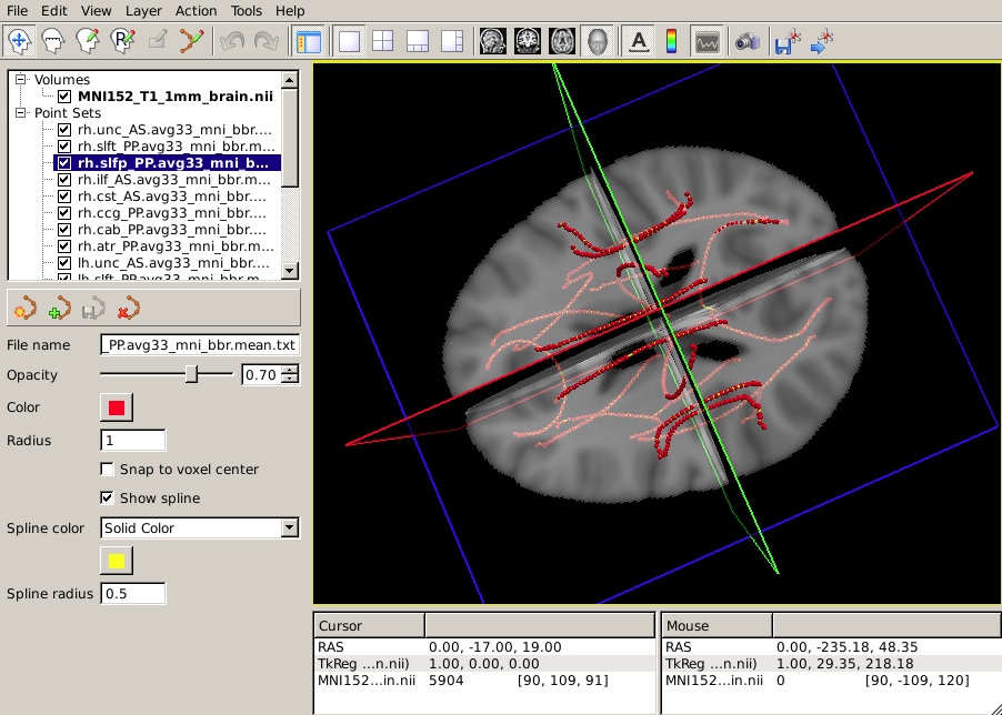
To view all 42 mean paths in template space, run the following:
freeview -v $FREESURFER_HOME/trctrain/hcp/MGH35_HCP_FA_template.nii.gz \
         -t $FREESURFER_HOME/trctrain/hcp/syn/*.mean.trk
You should see something like this in the 3D view:
The following information is based on hypothetical statistical data. The text file of p-values is not available so do not expect your end result to look identical to this image.
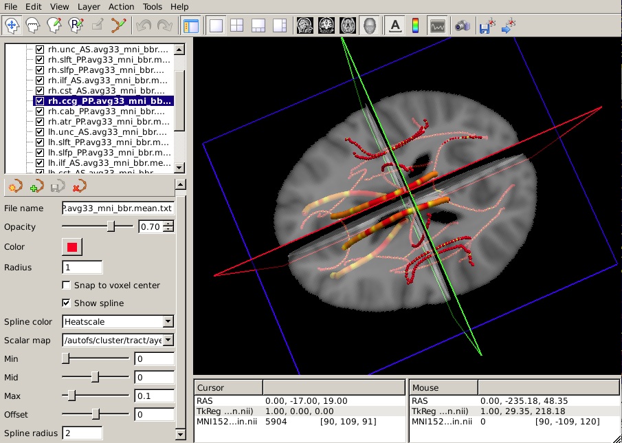
Let's say that you have performed a statistical analysis on your subjects in your statistical software of choice. If you save the p-values corresponding to each position along a tract to a simple text file, you can now display these p-values as a heat map on the corresponding mean path. (It is assumed that the number of p-values in your text file is equal to the number of points on the mean path, which is the same as the number of rows of values in the group tables produced by trac-all -stat. If not, display may be problematic.)
To display the p-values from your hypothetical analysis on one of the mean paths, do the following:
Select the mean path of your choice on the panel in the top left of the freeview window. On the left menu, click on Show spline.
From the Spline color menu, choose Heatscale.
From the Scalar map menu, choose Load... and select the text file that contains the p-values from your statistical analysis.
To hide the waypoints, which show up as small spheres, increase the Spline radius so that it is greater than the Radius of the waypoints. (In the example below, we have set the Spline radius to 2, while the Radius of the waypoints is 1.)
Set the Min, Mid, and Max of the heatscale to threshold the p-values as you wish.
You can do this for as many of the tracts as you have performed statistical analyses on. The end result will look something like this in the 3D view:
Summary
By the end of this page, you should know how to:
- Extract statistics (anisotropy and diffusivity measures), either averaged over an entire white-matter pathway, or as a function of position along the trajectory of the pathway
- Combine statistics into tables for group analysis
- Perform whole-tract and along-tract statistical analysis
- Visualize the outputs of along-tract statistical analysis in freeview
Quiz
You can test your knowledge of this tutorial by clicking here for a quiz!
Back to list of all tutorials | Back to course page | Previous