|
Size: 15279
Comment:
|
Size: 12971
Comment:
|
| Deletions are marked like this. | Additions are marked like this. |
| Line 1: | Line 1: |
| [wiki:Self:FsTutorial top] | [wiki:Self:FsTutorial/MorphAndRecon previous] | [wiki:Self:FsTutorial/Visualization next] == FreeSurfer Tutorial: Group Analysis (15 minutes of exercises) == Assuming that all surface reconstruction has been completed for all subjects in the study, FreeSurfer's mris_glm command can be used to perform inter-subject / group averaging and inference on the cortical surface. Mris_glm models the data as a linear combination of effects related to variables of interest, confounds and errors, and permits statistical inferences to be made about effects of interest in relation to error variance. For group analysis, this technique fits a general linear model (GLM) at each surface vertex to explain the data from all subjects in the study. In this section, a brief overview of linear modeling is presented and [https://surfer.nmr.mgh.harvard.edu/fswiki/mris_5fglm mris_glm] is described for estimating a linear model and testing hypotheses. The modeling overview can be skipped if this material is already familiar. Other software packages have similar types of programs (e.g., FSL's GFEAT). === 1.0 Preparing for Group Analysis === For group analysis, create an average subject from the surfaces of all the participants in the study. This average will be used as the target surface for group analysis on which the results can be output and viewed. To create this average, use ''make_average_surface'': {{{ make_average_surface --subjects <subj1> <subj2> ... }}} the default behavior of this script is to create a subject in the $SUBJECTS_DIR named 'average'. This behavior can be modified on the command line. An example of an average surface has been created for you and is saved in: $FREESURFER_HOME/subjects/buckner_public_distribution/FsTutorialDataSet/group_analysis_tutorial This average subject was created using the subjects found in: $FREESURFER_HOME/subjects/buckner_public_distribution/sample_group_study === 2.0 Linear Modeling overview === Linear modeling describes the observed data as a linear combination of explanatory factors plus noise, and determines how well that description explains the data being analyzed. For group morphometric analysis, the observed data is comprised of a set of surface measures (such as cortical thickness) at each vertex in a surface model, for each subject in the group. This data can be organized as a set of vectors, each associated with a different vertex in the surface model, and containing a surface measurement for every subject in the group at the corresponding vertex. First, a linear model must be designed to include all explanatory variables (EVs) that may account for each vector's values. A simple linear model is given by '''''y'''=a'''*x'''+b+'''e''''', where the observed data '''''y''''' is a one-dimensional vector of surface measures -- one measurement per subject at a vertex; '''''x''''' is a one-dimensional vector containing a variable, such as age, describing each subject; ''a'' is the parameter estimate (PE) for '''''x''''', for instance the value that a subject's age must be multiplied by to fit the data in '''''y'''''; ''b'' is a constant, and in this example, would correspond to the baseline measurement present in the data; and '''''e''''' is the error in the model fitting. If an additional explanatory variable is added to explain the observed data, the model would be given as '''''y'''=a1*'''x1'''+a2*'''x2'''+b+'''e''''', containing two different model waveforms, ''a1*'''x1''''' and ''a2*'''x2''''', corresponding to two variables, such as age and gender, describing all subjects in the study. '''2.1 Estimation overview''' [[BR]] Once the model is specified, an estimation step follows, in which the model is fit to each vertex's vector separately; no interactions between vertices are taken into account in the examples presented here. This step generates the estimate of the "goodness of fit" of each of the explanatory variables to each vector of surface measurements. Thus if a particular vertex responds strongly to the explanatory variable '''''x1''''', a large value for ''a1'' will be produced by model-fitting; if the data appears unrelated to '''''x2''''' then ''a2'' will have a very small value. This kind of linear modeling is commonly expressed in matrix notation, where the the matrix '''''X''''' contains all the explanatory variables (designed effects and confounds) in the model, and the matrix '''''A''''' contains all the PEs. The matrix '''''X''''' is also commonly called the ''design matrix'' and it can be user-specified in FreeSurfer in the form of an FSGD (FreeSurfer Group Descriptor) file, as the exercises below illustrate. Each column of '''''X''''' corresponds to a different explanatory variable (also called a regressor or a covariate). As typically formulated and solved, the estimation step produces a set of estimates of the PEs, which in turn are used in hypothesis testing. '''2.2 Inference overview''' [[BR]] Estimates of the PEs can be converted into statistical parametric maps, which are commonly visualized as a color-coded surface overlay. The overlay assigns each vertex a value based on the likelihood that the null hypothesis is false at that vertex. A linear combination of estimates of PEs is used to encode the particular hypothesis of interest. This encoding is accomplished with a user-specified ''contrast vector'', which assigns a contrast weight to each column of the design matrix. A simplest example of a contrast vector that tests the null hypothesis for the explanatory variable associated with the first design matrix column would be[ 1 0 0 0...]. To compute this particular contrast at each vertex, the PE value associated with the first design matrix column at that vertex is divided by the error in its estimate, yielding a t-value. The t-value provides a good measure confidence in the estimate of the PE value, and can be converted into a probability (P) or Z statistic at that vertex via a standard statistical transformation. T, P and Z values all convey the same information about how significantly the observed data is related to a given explanatory variable. A t-value map can be produced for each explanatory variable of interest. Each map indicates how strongly vertices on the surface are related to one explanatory variable. Parameter estimates can also be compared to see if one explanatory variable is more strongly related to the data than another. To encode this kind of hypothesis, one PE is subtracted from another using a "contrast" vector such as [1 -1 0 0 ...], a combined standard error is computed, and a new t-map is generated. In a similar fashion, to test for a more complicated collection of effects, a matrix of contrast weights can be specified. A more rigorous description of single and multiple linear regression and GLM, types of analyses, estimation and hypothesis testing is available at [http://www.statsoft.com/textbook/stglm.html http://www.statsoft.com/textbook/stglm.html]. === 3.0 Using mris_glm for estimating the linear model and hypothesis testing === As stated earlier, mris_glm performs inter-subject/group averaging and inference on the surface by fitting a linear model at each vertex. The model consists of subject parameters ('''e.g.''', age, gender, etc). The model is the same across all vertices, though the fit will probably be different at each vertex. To specify the model, a design matrix that represents the GLM must be created. While estimation and inference can be performed in a single call to mris_glm, the tasks can also be separated, which can be much more convenient. '''3.1 Using the FreeSurfer Group Descriptor file to create a design matrix''' [[BR]] The FreeSurfer Group Descriptor File (FSGDF) Format (Version 1) provides a way to describe a group of subjects and their accompanying data. This can include class membership and other continuous variables, for example gender or age. When it exists, the FSGDF is used by mris_glm, tksurfer and tkmedit. The FSGDF is more than just a way to specify the design matrix. It also keeps track of group membership and covariate definitions. This information is then used to help visualize the results. This is not possible when only a design matrix is used. The design matrix is created from the class and variable information in the FSGD file and from the type of design specified when running mris_glm (''i.e.'', DODS: different offset different slope; or DOSS: different offset same slope). The design matrix will consist of regressors for intercepts and regressors for slopes. Each class will have an intercept regressor. The intercept regressor is a vector with a 1 for each subject that is a member of the class and 0 otherwise. The slope regressors are handled differently depending upon whether DODS or DOSS is used. For DODS, each class will have a slope regressor for each variable. Like the intercept regressor, the slope regressor for a class will be 0 for subjects not in the class. For subjects in the class, the slope regressor will be the value of the variable. Each variable will have its own set of regressors. For DOSS, each variable will have a single regressor which will be independent of class. This regressor will just be a vector of the variable values listed in the FSGD file. For DODS, the total number of regressors will be (Nc+1)*Nv, where Nc is the number of classes and Nv is the number of variables. The first Nc regressors will be the intercepts for each class. The next Nc regressors will be the slopes for each class for the first variable, etc. For DODS, the total number of regressors will be Nc+Nv. The first Nc regressors will be the intercepts for each class. The next Nv regressors will be the slopes for each variable. '''3.1.1 Formatting the FSGDF and using it with mris_glm''' [[BR]] The FSGDF format uses tags to identify information, as shown below: {{{ Example of a legal file: ------------------------- cut here ------------------ GroupDescriptorFile 1 Title MyTitle Class Class1 plus blue CLASS Class2 circle green SomeTag Variables Age Weight IQ Input subjid1 Class1 10 100 1000 Input subjid2 Class2 20 200 2000 #Input subjid3 Class2 20 200 2000 DefaultVariable Age ------------------------- cut here ------------------ }}} The FSGDF is specified in the command-line for mris_glm with the following option: {{{ --fsgd fname <gd2mtx> }}} where ''gd2mtx'' is the method by which the group description is converted into a design matrix. Legal values for ''gd2mtx'' are: * ''doss'' (different offset, same slope): this will create a design matrix in which each class has its own offset but forces all classes to have the same slope. * ''dods'' (different offset, different slope): this value models each class with its own offset and slope. * ''none'': this value is used if neither of the previous models work for your particular analysis. Using this value requires that you specify the design matrix manually. Notes: * The first line of the file must be "Group``Descriptor``File 1". * ''Title'' is not necessary. This will be used for display. * ''Class'' only needs the class name, the next two items, if present, will be used in the display. * The third input will be treated as a comment, due to the ''#'' at the beginning of the line. * ''Default``Variable'' is the default variable for display. * ''Some``Tag'' is not a valid tag, so it will be ignored. General Rules: * Tags are NOT case sensitive. * Labels are case sensitive. * When multiple items appear on a line, they can be separated by any white space (i.e., blank or tab). * Any line where # appears as the first non-white space character is treated as a comment (ignored). * The ''Variables'' line should appear before the first Input line. * All Class lines should appear before the first Input line. * Variable label replications are not allowed. * Class label replications are not allowed. * Subject Id replications are not allowed. * If a class label is not used, a warning is printed out. * ''Default``Variable'' must be a member of the Variable list. * No error is generated if a tag does not match. * Empty lines are OK. * A class label can optionally be followed by a class marker. * A class marker can optionally be followed by a class color. '''3.1.2 An example FSGDF and design matrices for DODS and DOSS''' [[BR]] This similar FSGD file has two classes (Nc=2) and three variables (Nv=3): {{{ ------------------------- cut here ------------------ GroupDescriptorFile 1 Class Class1 CLASS Class2 Variables Age Weight IQ Input subjid1a Class1 10 100 1000 Input subjid1b Class1 15 150 1500 Input subjid2a Class2 20 200 2000 Input subjid2b Class2 25 250 2500 DefaultVariable Age ------------------------- cut here ------------------ }}} For DODS, the number of regressors is (Nc+1)*Nv=9, and the design matrix would be: {{{ 1 0 10 0 100 0 1000 0 1 0 15 0 150 0 1500 0 0 1 0 20 0 200 0 2000 0 1 0 25 0 250 0 2500 }}} For DOSS, the number of regressors is Nc+Nv=5, and the design matrix would be: {{{ 1 0 10 100 1000 1 0 15 150 1500 0 1 20 200 2000 0 1 25 250 2500 }}} '''3.2 Estimation exercises''' [[BR]] Consider the following table as an example of a small demographic dataset describing 42 subjects; the table lists subject Id, Age and Gender for each. In the following exercises, an FSGD file will be created to specify a design matrix that examines the relationship between a subject's age and cortical thickness for this dataset; the mris_glm command-line will be constructed to perform the estimation; and the output created from the estimation step will be noted. attachment:demoTable2.jpg * [wiki:Self:FsTutorial/CreateFSGDfile Exercise A. Create an FSGD file using the table above] * [wiki:Self:FsTutorial/PerformEstimation Exercise B. Construct command line for mris_glm to perform the estimation] '''3.3 Inference exercises''' [[BR]] Once parameter estimates have been generated, they can be used to determine how significantly any given explanatory variable is related to the data; they can also be compared to see if one explanatory variable is more strongly related to the data than another. The framework for testing specific hypotheses is specified in the form of a contrast vector. For instance, a contrast vector such as [1 0 0 0 ...] is used to examine the strength of the observed effect from the EV in the first design matrix column. Another contrast vector, such as [1 -1 0 0 ...], is used to compare the effects between the first two EVs in the design matrix. In the following examples, specific contrast vectors are formed, and used with mris_glm to compute the corresponding statistical results. * [wiki:Self:FsTutorial/CreateContrastVectors Exercise C. Specify contrast vectors to test hypotheses] * [wiki:Self:FsTutorial/ComputeContrast Exercise D. Construct command line for mris_glm to compute the contrast] |
[[FsTutorial|Back to Tutorial Top]] <<TableOfContents>> = Introduction = This tutorial is designed to introduce you to the "command-line" group analysis stream in FreeSurfer (as opposed to QDEC which is GUI-driven), including correction for multiple comparisons. While this tutorial shows you how to perform a surface-based thickness study, it is important to realize that most of the concepts learned here apply to any group analysis in FreeSurfer, surface or volume, thickness or fMRI. Here are some useful Group Analysis Links:<<BR>> [[FsTutorial/QdecGroupAnalysis|QDEC Tutorial]]<<BR>> [[FsgdFormat | FSGD Format]]<<BR>> [[FsgdExamples|FSGD Examples]]<<BR>> [[DodsDoss| DODS vs DOSS]]<<BR>> [[FsTutorial/GroupAnalysisJP|Old Group Analysis Tutorial]]<<BR>> = This Data Set = The data used for this tutorial is 40 subjects from Randy Buckner's lab. It consists of males and females ages 18 to 93. You can see the demographics [[FsTutorial/GroupAnalysisDemographics|here]]. You will perform an analysis looking for the effect of age on cortical thickness accounting for the effects of gender in the analysis. This is the same data set used in the [[FsTutorial/QdecGroupAnalysis|QDEC Tutorial]], and you will get the same result. = General Linear Model (GLM) DODS Setup = == Design Matrix/FSGD File == For this example, we will model the thickness as a straight line. A line has two parameters: intercept (or offset) and a slope. 1. The slope is the change of thickness with age 1. The intercept/offset is interpreted as the thickness at age=0. Parameter estimates are also called "regression coefficients". To account for effects of gender, we will model each sex with its own line, meaning that there will be four linear parameters (also called "betas"): 1. Intercept for Females 1. Intercept for Males 1. Slope for Females 1. Slope for Males In FreeSurfer, this type of design is called [[DodsDoss| DODS]] (for "Different-Offset, Different-Slope"). In FreeSurfer, you can either create your own design matrices, or, if you can specify your design in terms of a FreeSurfer Group Descriptor File [[FsgdFormat| (FSGD)]], FreeSurfer will create them for you. The FSGD file is a simple text file. See [[FsgdFormat|this page]] for the format. The [[FsTutorial/GroupAnalysisDemographics|demographics page]] also has an example FSGD file for this data. Things to do: 1. Create an FSGD file for the above design. One (gender_age.fsgd) already exists so that you can continue with the exercises. == Contrasts == A contrast is a vector that embodies the hypothesis we want to test. In this case, we wish to test the change in thickness with age after removing the effects of gender. To do this, create a simple text file with the following numbers: {{{ 0 0 0.5 0.5 }}} Notes: 1. There is one value for each parameter (so 4 values) 1. The intercept/offset values are 0 (nuisance) 1. The slope values are 0.5 so as to average the F and M slopes 1. A file called lh-Avg-thickness-age-Cor.mtx already exists = Analysis = == Assemble the Data (mris_preproc) == Assembling the data simply means: 1. Resampling each subject's data into a common space, and 1. Concatenating all the subjects' into a single file 1. Spatial smoothing (can be done between 1 and 2) This can be done in two equivalent ways: === Previously Cached (qcached) Data === When you have run recon-all with the -qcache option, recon-all will resample data onto the average subject (fsaverage) and smooth it at various FWHM (full-width/half-max), usually 0, 5, 10, 10, 20, and 25mm. This can speed later processing. The data for this tutorial have been cached, so run: {{{ mris_preproc --fsgd gender_age.fsgd \ --cache-in thickness.fwhm10.fsaverage \ --target fsaverage --hemi lh \ --out lh.gender_age.thickness.10.mgh }}} Notes: 1. Only takes a few seconds because the data have been cached 1. The FSGD file lists all the subjects, helps keep order. 1. The independent variable is the thickness smoothed to 10mm FWHM. 1. The data are for the left hemisphere 1. The output is lh.gender_age.thickness.10.mgh (which already exists) Things to do: 1. Run mri_info on lh.gender_age.thickness.10.mgh to find its dimensions. === Uncached Data === In the case that you have no cached the data, you can perform the same operations manually using the two commands below. There is no need to do this for this tutorial. {{{ OPTIONAL: THIS WILL TAKE ABOUT 10 MINUTES mris_preproc --fsgd gender_age.fsgd \ --target fsaverage --hemi lh \ --meas thickness \ --out lh.gender_age.thickness.00.mgh }}} Notes: 1. This resamples each subjects data to fsaverage 1. Output is lh.gender_age.thickness.00.mgh, which is unsmoothed {{{ OPTIONAL: THIS WILL TAKE ABOUT 5 MINUTES mri_surf2surf --hemi lh \ --s fsaverage \ --sval lh.gender_age.thickness.mgh \ --fwhm 10 \ --cortex \ --tval lh.gender_age.thickness.10B.mgh }}} 1. This smooths by 10mm FWHM 1. "--cortex" means only smooth areas in cortex (exclude medial wall). This is automatically done with qcache. You can also specify other labels. 1. Output is lh.gender_age.thickness.10B.mgh. == GLM Analysis (mri_glmfit) == {{{ mri_glmfit \ --y lh.gender_age.thickness.10.mgh \ --fsgd gender_age.fsgd dods\ --C lh-Avg-thickness-age-Cor.mtx \ --surf fsaverage lh \ --cortex \ --glmdir lh.gender_age.glmdir }}} Notes: 1. Input is lh.gender_age.thickness.10.mgh 1. Same FSGD used as with mris_preproc. Maintains subject order! 1. DODS is specified (it is the default) 1. Only one contrast is used (lh-Avg-thickness-age-Cor.mtx) but you can specify multiple contrasts. 1. "--cortex" specifies that the analysis only be done in cortex (ie, medial wall is zeroed out). Other labels can be used. 1. The output directory is lh.gender_age.glmdir 1. Should only take about 1min to run. Things to do: When this command is finished you will have an lh.gender_age.glmdir. There will be a number of output files in this directory, as well as two other directories. If you did an ''ls'' in your glmdir there will be: {{{ y.fsgd -- copy of input FSGD file (text) Xg.dat -- design matrix (text) mask.mgh -- binary mask (surface overlay) beta.mgh -- all parameter estimates (surface overlay) rstd.mgh -- residual standard deviation (surface overlay) sar1.mgh -- residual spatial AR1 (surface overlay) fwhm.dat -- average FWHM of residual (text) dof.dat -- degrees of freedom (text) lh-Avg-thickness-age-Cor -- contrast subdirectory mri_glmfit.log -- log file (text, send this with bug reports) }}} There will be a subdirectory for each contrast that you specify. The name of the directory will be that of the contrast matrix file (without the .mtx extension). The '''lh-Avg-thickness-age-Cor''' directory will have the following files: Study Questions: 1. What was the DOF for this experiment? 1. What was the FWHM? 1. How many frames does beta have? Why? Look at the contrast subdirectory: {{{ C.dat -- original contrast matrix (text) gamma.mgh -- contrast effect size (surface overlay) F.mgh -- F ratio of contrast (surface overlay) sig.mgh -- significance, -log10(pvalue), uncorrected (surface overlay) }}} View the uncorrected significance map with tksurfer: {{{ tksurfer fsaverage lh inflated \ -annot aparc.annot -fthresh 2 \ -overlay lh.gender_age.glmdir/sig.mgh \ }}} You should see: {{attachment:groupana.lat.uncor.th2.gif}} {{attachment:groupana.med.uncor.th2.gif}} Notes: 1. The threshold is set to 2, meaning vertices with p<.01, uncorrected, will have color. 1. Blue means a negative correlation (thickness decreases with age), red is positive correlation. 1. Click on a point in the Precentral Gyrus. What is it's value? What does it mean? Viewing the medial surface, change the overlay threshold to something very, very low (say, .01): {{{ View->Configure->Overlay, set "Min" .01 }}} You should see: {{attachment:groupana.med.uncor.th0.gif}} Notes: 1. Almost all of cortex now has color 1. The non-cortical areas are still blank (0) because they were excluded with --cortex in mri_glmfit above. == Clusterwise Correction for Multiple Comparisons == To perform a cluster-wise correction for multiple comparisons, we will run a simulation. The simulation is a way to get a measure of the distribution of the maximum cluster size under the null hypothesis. This is done by iterating over the following steps: 1. Synthesize a z map 1. Smooth z map (using residual FWHM) 1. Threshold z map (level and sign) 1. Find clusters in thresholded map 1. Record area of maximum cluster 1. Repeat over desired number of iterations (usually > 5000) In FreeSurfer, this information is stored in a simple text file called a CSD (Cluster Simulation Data). Once we have the distribution of the maximum cluster size, we correct for multiple comparisons by: 1. Going back to the original data 1. Thresholding using same level and sign 1. Finding clusters in thresholded map 1. For each cluster, p = probability of seeing a maximum cluster that size or larger during simulation. === Run the simulation === All these steps are performed with the mri_glmfit-sim: {{{ mri_glmfit-sim \ --glmdir lh.gender_age.glmdir \ --sim mc-z 5 4 mc-z.negative \ --sim-sign neg \ --overwrite }}} Notes: 1. Specify the same GLM directory (--glmdir) 1. The simulation type is Z Monte Carlo (mc-z) 1. Specify the sign (neg for negative, pos, or abs) 1. Vertex-wise thershold of 4 (p < .0001) 1. Only 5 iterations (usually > 5000) 1. CSD files will have mc-z.negative base 1. --overwrite deletes previous CSD files This has been run this data with 1000 iterations (CSD base of mc-z.neg). This can often take many hours. === View CSD File === The CSD files are stored in lh.gender_age.glmdir/csd. Look at one of them: {{{ less lh.gender_age.glmdir/csd/mc-z.neg4.j001-lh-Avg-thickness-age-Cor.csd }}} Or click [[FsTutorial/GroupAnalysisCsd|here]]. Notes: 1. Rows that begin with '#' are headers or comments. 1. Each data row is an iteration. 1. The 3rd column is the maximum cluster size for that iteration. 1. The CSD file itself is not particularly important, so don't worry too much about it. === View the Corrected Results === In the contrast subdirectory, you will see several new files, all beginning with mc-z: {{{ mc-z.neg4.sig.cluster.summary - summary of clusters (text) mc-z.neg4.sig.cluster.mgh - cluster-wise corrected map (overlay) mc-z.neg4.sig.ocn.annot - annotation of clusters }}} First, look at the cluster summary (or click [[FsTutorial/GroupAnalysisClusterSummary|here]]): {{{ less lh.gender_age.glmdir/lh-Avg-thickness-age-Cor.csd/mc-z.neg4.sig.cluster.summary }}} Notes: 1. This is a list of all the clusters that were found (38 of them) 1. The CWP column is the cluster-wise probability (the number you are interested in). It is a simple p (ie, NOT -log10(p)). 1. Note that ALL clusters, regardless of their significance. 1. Cluster number 1 has a CWP of p=.001. 1. Cluster number 21 has a CWP of p=.007. Load the cluster annotation in tksurfer {{{ tksurfer fsaverage lh inflated \ -annot lh.gender_age.glmdir/lh-Avg-thickness-age-Cor.csd/mc-z.neg4.sig.ocn.annot \ -fthresh 2 }}} You should see: {{attachment:groupana.lat.clusters.gif}} {{attachment:groupana.med.clusters.gif}} Notes: 1. These are all clusters, regardless of significance. 1. When you click on a cluster, the label will tell you the cluster number (eg, cluster-021). Change the label mode to "Outline" by hitting the outline button {{attachment:tksurfer.outline.gif}}. Now load the cluster p-value overlay with {{{ File->LoadOverlay "Browse..." Select mc-z.neg4.sig.cluster.mgh OK OK }}} You should see: {{attachment:groupana.lat.cor.th2.gif}} {{attachment:groupana.med.cor.th2.gif}} Note: Things to do: 1. Find and click on cluster 1. It is blue and has a value of -3 since this is -log10(.001). The -3 is because the correlation is negative. 1. Find and click on cluster 21. Its value is -1.11 because this is -log10(.007). Note that it is transparent because its significance is worse than the threshold we set (-fthresh 2, p < .01). 1. All vertices within a cluster are the same value (the p-value of the cluster). 1. You can changed the cluster-wise threshold by clicking on View->Configure->Overlay, and setting the "Min" to your desired level. As you do this, some clusters will change transparency. |
Introduction
This tutorial is designed to introduce you to the "command-line" group analysis stream in FreeSurfer (as opposed to QDEC which is GUI-driven), including correction for multiple comparisons. While this tutorial shows you how to perform a surface-based thickness study, it is important to realize that most of the concepts learned here apply to any group analysis in FreeSurfer, surface or volume, thickness or fMRI.
Here are some useful Group Analysis Links:<<BR>> QDEC Tutorial
FSGD Format
FSGD Examples
DODS vs DOSS
Old Group Analysis Tutorial
This Data Set
The data used for this tutorial is 40 subjects from Randy Buckner's lab. It consists of males and females ages 18 to 93. You can see the demographics here. You will perform an analysis looking for the effect of age on cortical thickness accounting for the effects of gender in the analysis. This is the same data set used in the QDEC Tutorial, and you will get the same result.
General Linear Model (GLM) DODS Setup
Design Matrix/FSGD File
For this example, we will model the thickness as a straight line. A line has two parameters: intercept (or offset) and a slope.
- The slope is the change of thickness with age
- The intercept/offset is interpreted as the thickness at age=0.
Parameter estimates are also called "regression coefficients".
To account for effects of gender, we will model each sex with its own line, meaning that there will be four linear parameters (also called "betas"):
- Intercept for Females
- Intercept for Males
- Slope for Females
- Slope for Males
In FreeSurfer, this type of design is called DODS (for "Different-Offset, Different-Slope").
In FreeSurfer, you can either create your own design matrices, or, if you can specify your design in terms of a FreeSurfer Group Descriptor File (FSGD), FreeSurfer will create them for you. The FSGD file is a simple text file. See this page for the format. The demographics page also has an example FSGD file for this data.
Things to do:
- Create an FSGD file for the above design. One (gender_age.fsgd) already exists so that you can continue with the exercises.
Contrasts
A contrast is a vector that embodies the hypothesis we want to test. In this case, we wish to test the change in thickness with age after removing the effects of gender. To do this, create a simple text file with the following numbers:
0 0 0.5 0.5
Notes:
- There is one value for each parameter (so 4 values)
- The intercept/offset values are 0 (nuisance)
- The slope values are 0.5 so as to average the F and M slopes
- A file called lh-Avg-thickness-age-Cor.mtx already exists
Analysis
Assemble the Data (mris_preproc)
Assembling the data simply means:
- Resampling each subject's data into a common space, and
- Concatenating all the subjects' into a single file
- Spatial smoothing (can be done between 1 and 2)
This can be done in two equivalent ways:
Previously Cached (qcached) Data
When you have run recon-all with the -qcache option, recon-all will resample data onto the average subject (fsaverage) and smooth it at various FWHM (full-width/half-max), usually 0, 5, 10, 10, 20, and 25mm. This can speed later processing. The data for this tutorial have been cached, so run:
mris_preproc --fsgd gender_age.fsgd \
  --cache-in thickness.fwhm10.fsaverage \
  --target fsaverage --hemi lh \
  --out lh.gender_age.thickness.10.mgh
Notes:
- Only takes a few seconds because the data have been cached
- The FSGD file lists all the subjects, helps keep order.
- The independent variable is the thickness smoothed to 10mm FWHM.
- The data are for the left hemisphere
- The output is lh.gender_age.thickness.10.mgh (which already exists)
Things to do:
- Run mri_info on lh.gender_age.thickness.10.mgh to find its dimensions.
Uncached Data
In the case that you have no cached the data, you can perform the same operations manually using the two commands below. There is no need to do this for this tutorial.
OPTIONAL: THIS WILL TAKE ABOUT 10 MINUTES
mris_preproc --fsgd gender_age.fsgd \
  --target fsaverage --hemi lh \
  --meas thickness \
  --out lh.gender_age.thickness.00.mgh
Notes:
- This resamples each subjects data to fsaverage
- Output is lh.gender_age.thickness.00.mgh, which is unsmoothed
OPTIONAL: THIS WILL TAKE ABOUT 5 MINUTES
mri_surf2surf --hemi lh \
  --s fsaverage \
  --sval lh.gender_age.thickness.mgh \
  --fwhm 10 \
  --cortex \
  --tval lh.gender_age.thickness.10B.mgh
- This smooths by 10mm FWHM
- "--cortex" means only smooth areas in cortex (exclude medial wall). This is automatically done with qcache. You can also specify other labels.
- Output is lh.gender_age.thickness.10B.mgh.
GLM Analysis (mri_glmfit)
mri_glmfit \
  --y lh.gender_age.thickness.10.mgh \
  --fsgd gender_age.fsgd dods\
  --C lh-Avg-thickness-age-Cor.mtx \
  --surf fsaverage lh \
  --cortex \
  --glmdir lh.gender_age.glmdir
Notes:
- Input is lh.gender_age.thickness.10.mgh
- Same FSGD used as with mris_preproc. Maintains subject order!
- DODS is specified (it is the default)
- Only one contrast is used (lh-Avg-thickness-age-Cor.mtx) but you can specify multiple contrasts.
- "--cortex" specifies that the analysis only be done in cortex (ie, medial wall is zeroed out). Other labels can be used.
- The output directory is lh.gender_age.glmdir
- Should only take about 1min to run.
Things to do:
When this command is finished you will have an lh.gender_age.glmdir. There will be a number of output files in this directory, as well as two other directories. If you did an ls in your glmdir there will be:
y.fsgd -- copy of input FSGD file  (text)
Xg.dat -- design matrix  (text)
mask.mgh -- binary mask (surface overlay)
beta.mgh -- all parameter estimates (surface overlay)
rstd.mgh -- residual standard deviation (surface overlay)
sar1.mgh -- residual spatial AR1  (surface overlay)
fwhm.dat -- average FWHM of residual (text)
dof.dat  -- degrees of freedom (text)
lh-Avg-thickness-age-Cor -- contrast subdirectory
mri_glmfit.log -- log file (text, send this with bug reports)
There will be a subdirectory for each contrast that you specify. The name of the directory will be that of the contrast matrix file (without the .mtx extension). The lh-Avg-thickness-age-Cor directory will have the following files:
Study Questions:
- What was the DOF for this experiment?
- What was the FWHM?
- How many frames does beta have? Why?
Look at the contrast subdirectory:
C.dat -- original contrast matrix (text)
gamma.mgh -- contrast effect size (surface overlay)
F.mgh -- F ratio of contrast  (surface overlay)
sig.mgh -- significance, -log10(pvalue), uncorrected (surface overlay)
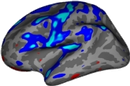
View the uncorrected significance map with tksurfer:
tksurfer fsaverage lh inflated \
  -annot aparc.annot -fthresh 2 \
  -overlay lh.gender_age.glmdir/sig.mgh \
You should see:
![]()
![]()
Notes:
The threshold is set to 2, meaning vertices with p<.01, uncorrected, will have color.
- Blue means a negative correlation (thickness decreases with age), red is positive correlation.
- Click on a point in the Precentral Gyrus. What is it's value? What does it mean?
Viewing the medial surface, change the overlay threshold to something very, very low (say, .01):
View->Configure->Overlay, set "Min" .01
You should see:
![]()
Notes:
- Almost all of cortex now has color
- The non-cortical areas are still blank (0) because they were excluded with --cortex in mri_glmfit above.
Clusterwise Correction for Multiple Comparisons
To perform a cluster-wise correction for multiple comparisons, we will run a simulation. The simulation is a way to get a measure of the distribution of the maximum cluster size under the null hypothesis. This is done by iterating over the following steps:
- Synthesize a z map
- Smooth z map (using residual FWHM)
- Threshold z map (level and sign)
- Find clusters in thresholded map
- Record area of maximum cluster
Repeat over desired number of iterations (usually > 5000)
In FreeSurfer, this information is stored in a simple text file called a CSD (Cluster Simulation Data).
Once we have the distribution of the maximum cluster size, we correct for multiple comparisons by:
- Going back to the original data
- Thresholding using same level and sign
- Finding clusters in thresholded map
- For each cluster, p = probability of seeing a maximum cluster that size or larger during simulation.
Run the simulation
All these steps are performed with the mri_glmfit-sim:
mri_glmfit-sim \
  --glmdir lh.gender_age.glmdir \
  --sim mc-z 5 4 mc-z.negative \
  --sim-sign neg \
  --overwrite
Notes:
- Specify the same GLM directory (--glmdir)
- The simulation type is Z Monte Carlo (mc-z)
- Specify the sign (neg for negative, pos, or abs)
Vertex-wise thershold of 4 (p < .0001)
Only 5 iterations (usually > 5000)
- CSD files will have mc-z.negative base
- --overwrite deletes previous CSD files
This has been run this data with 1000 iterations (CSD base of mc-z.neg). This can often take many hours.
View CSD File
The CSD files are stored in lh.gender_age.glmdir/csd. Look at one of them:
less lh.gender_age.glmdir/csd/mc-z.neg4.j001-lh-Avg-thickness-age-Cor.csd
Or click here.
Notes:
- Rows that begin with '#' are headers or comments.
- Each data row is an iteration.
- The 3rd column is the maximum cluster size for that iteration.
- The CSD file itself is not particularly important, so don't worry too much about it.
View the Corrected Results
In the contrast subdirectory, you will see several new files, all beginning with mc-z:
mc-z.neg4.sig.cluster.summary - summary of clusters (text)
mc-z.neg4.sig.cluster.mgh - cluster-wise corrected map (overlay)
mc-z.neg4.sig.ocn.annot - annotation of clusters
First, look at the cluster summary (or click here):
less lh.gender_age.glmdir/lh-Avg-thickness-age-Cor.csd/mc-z.neg4.sig.cluster.summary
Notes:
- This is a list of all the clusters that were found (38 of them)
- The CWP column is the cluster-wise probability (the number you are interested in). It is a simple p (ie, NOT -log10(p)).
- Note that ALL clusters, regardless of their significance.
- Cluster number 1 has a CWP of p=.001.
- Cluster number 21 has a CWP of p=.007.
Load the cluster annotation in tksurfer
tksurfer fsaverage lh inflated \
  -annot  lh.gender_age.glmdir/lh-Avg-thickness-age-Cor.csd/mc-z.neg4.sig.ocn.annot \
  -fthresh 2
You should see:
![]()
![]()
Notes:
- These are all clusters, regardless of significance.
- When you click on a cluster, the label will tell you the cluster number (eg, cluster-021).
Change the label mode to "Outline" by hitting the outline button  . Now load the cluster p-value overlay with
  File->LoadOverlay
  "Browse..."
  Select  mc-z.neg4.sig.cluster.mgh
  OK
  OK
You should see:
![]()
![]()
Note:
Things to do:
- Find and click on cluster 1. It is blue and has a value of -3 since this is -log10(.001). The -3 is because the correlation is negative.
- Find and click on cluster 21. Its value is -1.11 because this is -log10(.007). Note that it is transparent because its significance
is worse than the threshold we set (-fthresh 2, p < .01).
- All vertices within a cluster are the same value (the p-value of the cluster).
- You can changed the cluster-wise threshold by clicking on
View->Configure->Overlay, and setting the "Min" to your desired level. As you do this, some clusters will change transparency.