|
Size: 20914
Comment: updated sig.mgh screenshots
|
← Revision 67 as of 2024-04-24 17:02:50 ⇥
Size: 18284
Comment:
|
| Deletions are marked like this. | Additions are marked like this. |
| Line 3: | Line 3: |
| [[FsTutorial|Back to course page]] <<TableOfContents(1)>> |
[[VirtualCourse|Back to course page]] = Surface Based Group Analysis = |
| Line 8: | Line 10: |
| Line 12: | Line 15: |
| ''To copy: Highlight the command in the box above, right click and select copy (or use keyboard shortcut Ctrl+c), then use the middle button of your mouse to click inside the terminal window (this will paste the command). Press enter to run the command.'' | ''To copy: Highlight the command in the box above, right click and select copy (or use keyboard shortcut Ctrl+c), then use the middle button of your mouse to click inside the terminal window to paste the command (or use keyboard shortcut Ctrl+Shift+v). Press enter to run the command.'' |
| Line 14: | Line 18: |
| Line 16: | Line 21: |
| Line 29: | Line 35: |
| Line 30: | Line 37: |
| Line 32: | Line 40: |
| This tutorial is designed to introduce you to the "command-line" group analysis stream in FreeSurfer (as opposed to QDEC which is GUI-driven), including correction for multiple comparisons. While this tutorial shows you how to perform a surface-based thickness study, it is important to realize that most of the concepts learned here apply to any group analysis in FreeSurfer, surface or volume, thickness or fMRI. Here are some useful Group Analysis links you might want to refer back to at a later time: <<BR>> [[FsTutorial/QdecGroupAnalysis_freeview|QDEC Tutorial]]<<BR>> [[FsgdFormat|FSGD Format]]<<BR>> [[FsgdExamples|FSGD Examples]]<<BR>> [[DodsDoss|DODS vs DOSS]]<<BR>> ## [[FsTutorial/GroupAnalysisJP|Old Group Analysis Tutorial]]<<BR>> |
This tutorial is designed to introduce you to the "command-line" group analysis stream in !FreeSurfer. While this tutorial shows you how to perform a surface-based thickness study, it is important to realize that most of the concepts learned here apply to any group analysis in !FreeSurfer, surface, volume, thickness or fMRI. Here are some useful Group Analysis links you might want to refer back to at a later time: <<BR>> [[FsgdFormat|FSGD Format]]<<BR>> [[FsgdExamples|FSGD Examples]]<<BR>> [[DodsDoss|DODS vs DOSS]]<<BR>> |
| Line 36: | Line 43: |
| The data used for this tutorial is 40 subjects from Randy Buckner's lab. It consists of males and females, ages 18 to 93. You can see the demographics [[FsTutorial/GroupAnalysisDemographics|here]]. You will perform an analysis looking for the effect of age on cortical thickness, accounting for the effects of gender in the analysis. This is the same data set used in the [[FsTutorial/QdecGroupAnalysis_freeview|QDEC Tutorial]], and you will get the same result. | The data used for this tutorial is 40 subjects from Randy Buckner's lab. It consists of males and females, ages 18 to 93. You can see the demographics [[FsTutorial/GroupAnalysisDemographics|here]]. You will perform an analysis looking for the effect of age on cortical thickness, accounting for the effects of gender in the analysis. |
| Line 39: | Line 47: |
| In this tutorial, we will model the thickness as a straight line. A line has two parameters: intercept (or offset) and a slope. For this example: | In this tutorial, we will model the thickness as a straight line. A line has two parameters: an intercept (or offset) and a slope. For this example: |
| Line 42: | Line 51: |
| Parameter estimates are also called "regression coefficients". To account for effects of gender, we will model each sex with its own line, meaning that there will be four linear parameters (also called "betas"): |
Parameter estimates are also called "regression coefficients" or "betas". To account for effects of gender, we will model each sex with its own line, meaning that there will be four linear parameters: |
| Line 48: | Line 58: |
| Line 49: | Line 60: |
| Line 50: | Line 62: |
| Things to do: | Exercises to try on your own: |
| Line 52: | Line 66: |
| Line 53: | Line 68: |
You can open the FSGD file for this tutorial (gender_age.fsgd) in a text editor such as gedit (for Linux) or open -e (for Macs). |
|
| Line 54: | Line 72: |
| A contrast is a vector that embodies the hypothesis we want to test. In this case, we wish to test the change in thickness with age, after removing the effects of gender. To do this, create a simple text file with the following numbers: | A contrast is a vector that embodies the hypothesis we want to test. In this case, we wish to test the change in thickness with age, after removing the effects of gender. To do this, create a simple text file with the following numbers (if you're using the tutorial data, this has already been done for you): |
| Line 59: | Line 78: |
| 1. There is one value for each parameter (so 4 values). 1. The intercept/offset values are 0 (nuisance). 1. The slope values are 0.5 so as to average the F and M slopes. 1. You'll find we created the contrast matrix for you already for this tutorial. It's a file called lh-Avg-thickness-age-Cor.mtx. (You will need to create your own contrast matrix when testing your own hypotheses on your data. !FreeSurfer doesn't automatically create this file.) |
1. Remember that for an analysis between two groups each with an intercept of b and a slope of m, the contrast matrix will be in the format [b1 b2 m1 m2]. 1. There is one value for each parameter (so 4 values total). 1. The intercept/offset values (b1, b2) are 0 (nuisance). 1. The slope values (m1, m2) are 0.5 so as to average the Female and Male slopes. 1. You'll find we created the contrast matrix for you already for this tutorial. It's a file called lh-Avg-thickness-age-Cor.mtx. You will need to create your own contrast matrix when testing your own hypotheses on your data. !FreeSurfer doesn't automatically create this file. There are examples of FSGD files and contrast matrices for many different hypotheses [[FsgdExamples|here]]. Open the contrast matrix file (lh-Avg-thickness-age-Cor.mtx) in a text editor. Remember, this file is located in the glm directory. |
| Line 65: | Line 89: |
| Line 68: | Line 93: |
| This can be done in two equivalent ways: == Previously Cached (qcached) Data == When you run recon-all with the -qcache option, recon-all will resample data onto the average subject (called fsaverage) and smooth it at various FWHM (full-width/half-max) values, usually 0, 5, 10, 15, 20, and 25mm. This can speed later processing. The data for this tutorial was ran with the -qcache option, so the FWHM are already cached. Run this command to assemble your previously cached data: {{{ mris_preproc --fsgd gender_age.fsgd \ --cache-in thickness.fwhm10.fsaverage \ --target fsaverage \ --hemi lh \ --out lh.gender_age.thickness.10.mgh }}} ---- '''NOTE''': The backslash allows you to copy and paste multiple lines of code as one command. We use this throughout the tutorials to display the commands in a more easy-to-read manner, while still allowing you to copy and paste. Whenever you are typing in your own commands, instead of copying and pasting a command written out across multiple lines, a backslash is not necessary. ---- Notes: 1. Only takes a few seconds because the data have been cached. 1. The FSGD file lists all the subjects, helps keep order. 1. The independent variable is the thickness smoothed to 10mm FWHM. 1. The target is the average subject, fsaverage. This subject is included with the !FreeSurfer distribution. 1. The data are for the left hemisphere. 1. Since the data is already cached, this {{{mris_preproc}}} command just creates a stack of all the smoothed thickness data from each subject into one file as output. 1. The output of this command is given by the --out flag. Here we call it '''lh.gender_age.thickness.10.mgh'''. Things to do: 1. Run mri_info on lh.gender_age.thickness.10.mgh to find its dimensions: {{{ mri_info lh.gender_age.thickness.10.mgh }}} |
|
| Line 95: | Line 95: |
| In the case that you have not cached the data, you can perform the same operations manually using the two commands below. These two commands give the equivalent results as running recon-all with -qcache. However, the commands below only create output for unsmoothed data and data smoothed to 10mm FWHM. qcache, on the other hand, smooths the data for a range of different FWHM vaules. '''THESE NEXT TWO COMMANDS ARE OPTIONAL FOR THE TUTORIAL, AND WILL TAKE ABOUT 10 MINUTES TO RUN. ''' ''' The tutorial data has already been pre-processed (cached) for you.''' |
In the case that you have not cached the data, you can use the two commands below. The commands below only create output for unsmoothed data and data smoothed to 10mm FWHM. ##'''THESE NEXT TWO COMMANDS ARE OPTIONAL FOR THE TUTORIAL, AND WILL TAKE ABOUT 5 MINUTES TO RUN. ''' ''' ''' ##''The tutorial data has already been pre-processed (cached) for you.''' {{{#!wiki caution '''Do not run these commands if you're at an organized course.''' It can take a while and the data has already been pre-processed for you. }}} |
| Line 106: | Line 112: |
| Line 108: | Line 115: |
| ##'''OPTIONAL: THIS WILL TAKE ABOUT 5 MINUTES''' | |
| Line 115: | Line 122: |
| --tval lh.gender_age.thickness.10B.mgh | --tval lh.gender_age.thickness.10.mgh |
| Line 119: | Line 126: |
| 1. Output is lh.gender_age.thickness.10B.mgh. (We have named the output file ...10B.mgh because the precreated file from running qcache ...10.mgh already exists.) | 1. "--sval" is the name of the source subject found in the $SUBJECTS_DIR. This input data must be sampled onto this subject's surface. 1. "--tval" is the name of the file where the data on the target surface will be stored. 1. Output is lh.gender_age.thickness.10.mgh. |
| Line 124: | Line 134: |
| --fsgd gender_age.fsgd dods\ | --fsgd gender_age.fsgd dods \ |
| Line 131: | Line 141: |
| Line 138: | Line 149: |
| 1. For more information about mri_glmfit, [[mri_glmfit|click here]] |
|
| Line 139: | Line 152: |
| Line 140: | Line 154: |
| Line 144: | Line 159: |
| Line 160: | Line 176: |
| Study Questions: 1. What was the DOF for this experiment? 1. What was the FWHM? 1. How many frames does beta have? Why? (hint: run mri_info on lh.gender_age.glmdir/beta.mgh) |
Notes: 1. The DOF is the degrees of freedom for the analysis which has important implications for calculating the p-value. 1. The FWHM is a measure of the smoothness of the data. Part of this comes from the applied smoothing (eg, 5mm FWHM) and part of the smoothness comes from the inherent smoothness in the data. When correcting for multiple comparisons, the final FWHM must be taken into account (but this is done automatically). |
| Line 165: | Line 183: |
| Line 169: | Line 188: |
| Line 182: | Line 202: |
| Line 186: | Line 207: |
| {{{ freeview -f $SUBJECTS_DIR/fsaverage/surf/lh.inflated:annot=aparc.annot:annot_outline=1:overlay=lh.gender_age.glmdir/lh-Avg-thickness-age-Cor/sig.mgh:overlay_threshold=4,5 -viewport 3d }}} |
{{{ freeview -f $SUBJECTS_DIR/fsaverage/surf/lh.inflated:annot=aparc.annot:annot_outline=1:overlay=lh.gender_age.glmdir/lh-Avg-thickness-age-Cor/sig.mgh:overlay_threshold=4,5 -viewport 3d -layout 1 }}} This command opens the left hemisphere inflated surface with the aparc annotation shown as an outline. The overlay sig.mgh is also loaded with a threshold of 4. |
| Line 190: | Line 214: |
| Line 191: | Line 216: |
| Notes: 1. The threshold is set to 4, meaning vertices with p<.0001, uncorrected, will have color. 1. Blue means a negative correlation (thickness decreases with age), red is positive correlation. |
This figure displays the correlation between age and cortical thickness with a threshold of 4. Notes: 1. The threshold is set to 4, meaning vertices with p<.0001, uncorrected, will have color. This threshold is equal to the -log(p-value). In this case, any vertex with a value under 4 will not be displayed in color, however the value will still be readable in the cursor/mouse section of freeview. 1. The lower threshold sets the minimum sigificance that a voxel must meet in order to be visible. It should be set such that only likely true effects will be seen. You can kind of think of it as a filter that removes voxels where no effect is present. The upper is just used for visualization purposes. If you set it very close to the min, then all voxels will appear to be the same color. If you set it higher, then you can get some gradation due to the strength of the effect. So the min removes voxels without an effect and the max allows you to see how the strength of the effect varies across the brain. 1. Blue represents a negative correlation (i.e. thickness decreases with age), red represents positive correlation (i.e. thickness increases with age). 1. In this example, the sig.mgh is used as the overlay and in practice this is what is normally used. However, the pcc.mgh can also be used as the overlay if it was created in the analysis. |
| Line 195: | Line 226: |
| Line 196: | Line 228: |
| Line 197: | Line 230: |
| {{attachment:glm3_fv5.3.jpg||height="370"}} Notes: |
{{attachment:lh-Avg_thickness-age-Cor-sig.mgh-0.01thresh.jpg||height="370"}} This figure displays the correlation between age and cortical thickness with a threshold of 0.01. Notes: |
| Line 201: | Line 239: |
| Line 202: | Line 241: |
| {{{ freeview -f $SUBJECTS_DIR/fsaverage/surf/lh.inflated:annot=aparc.annot:annot_outline=1:overlay=lh.gender_age.glmdir/lh-Avg-thickness-age-Cor/F.mgh:overlay_threshold=20,50 -viewport 3d |
{{{ freeview -f $SUBJECTS_DIR/fsaverage/surf/lh.inflated:annot=aparc.annot:annot_outline=1:overlay=lh.gender_age.glmdir/lh-Avg-thickness-age-Cor/F.mgh:overlay_threshold=20,50 -viewport 3d -layout 1 |
| Line 206: | Line 246: |
| = Clusterwise Correction for Multiple Comparisons = Note: The method used is based on: [[http://www.ncbi.nlm.nih.gov/pubmed/17011792|Smoothing and cluster thresholding for cortical surface-based group analysis of fMRI data. Hagler DJ Jr, Saygin AP, Sereno MI. NeuroImage (2006)]]. ==== Remember to run the following commands in every new terminal window (aka shell) you open throughout this tutorial (see top of page for detailed instructions): ==== If You're at an Organized Course: {{{ export SUBJECTS_DIR=$TUTORIAL_DATA/buckner_data/tutorial_subjs/group_analysis_tutorial cd $SUBJECTS_DIR/glm }}} If You're Not at an Organized Course: {{{ ## bash <source_freesurfer> export TUTORIAL_DATA=<path_to_your_tutorial_data> export SUBJECTS_DIR=$TUTORIAL_DATA/buckner_data/tutorial_subjs/group_analysis_tutorial cd $SUBJECTS_DIR/glm ## tcsh source $FREESURFER_HOME/SetUpFreeSurfer.csh setenv TUTORIAL_DATA <path_to_your_tutorial_data> setenv SUBJECTS_DIR $TUTORIAL_DATA/buckner_data/tutorial_subjs/group_analysis_tutorial cd $SUBJECTS_DIR/glm }}} -------- To perform a cluster-wise correction for multiple comparisons, we will run a simulation. The simulation is a way to get a measure of the distribution of the maximum cluster size under the null hypothesis. This is done by iterating over the following steps: 1. Synthesize a z map. 1. Smooth z map (using residual FWHM). 1. Threshold z map (level and sign). 1. Find clusters in thresholded map. 1. Record area of maximum cluster. 1. Repeat over desired number of iterations (usually > 5,000). In !FreeSurfer, this information is stored in a simple text file called a CSD (Cluster Simulation Data) file. Once we have the distribution of the maximum cluster size, we correct for multiple comparisons by: 1. Going back to the original data. 1. Thresholding using same level and sign. 1. Finding clusters in thresholded map. 1. For each cluster, p = probability of seeing a maximum cluster that size or larger during simulation. == Run the simulation == All these steps are performed with the command mri_glmfit-sim: {{{ mri_glmfit-sim \ --glmdir lh.gender_age.glmdir \ --cache 4 neg \ --cwp 0.05\ --2spaces }}} Notes: 1. Specify the same GLM directory (--glmdir). 1. Use precomputed Z Monte Carlo simulation (--cache). 1. Vertex-wise/cluster-forming threshold of 4 (p < .0001). 1. Specify the sign ("neg" for negative, "pos" for positive, or "abs" for absolute/unsigned). 1. --cwp 0.05 : Keep clusters that have cluster-wise p-values < 0.05. To see all clusters, set to .999. 1. --2spaces : adjust p-values for two hemispheres (this assumes you will eventually look at the right hemisphere too). 1. You can also generate your own precomputed data, but you only need to do this if you have a different average subject or you are not looking over all of the cortex. 1. You can also use a permutation simulation instead of Z Monte Carlo. Run mri_glmfit-sim --help to get more information. == View the Corrected Results == In the contrast subdirectory, you will see several new files by running: {{{ ls lh.gender_age.glmdir/lh-Avg-thickness-age-Cor }}} You will see the following new files: {{{ cache.th40.neg.sig.pdf.dat -- probability distribution function of clusterwise correction cache.th40.neg.sig.cluster.mgh -- cluster-wise corrected map (overlay) cache.th40.neg.sig.cluster.summary -- summary of clusters (text) cache.th40.neg.sig.masked.mgh -- uncorrected sig values masked by the clusters that survive correction cache.th40.neg.sig.ocn.annot -- output cluster number (annotation of clusters) cache.th40.neg.sig.ocn.mgh -- output cluster number (segmentation showing where each numbered cluster is) cache.th40.neg.sig.voxel.mgh -- voxel-wise map corrected for multiple comparisons at a voxel (rather than cluster) level cache.th40.neg.sig.y.ocn.dat -- the average value of each subject in each cluster }}} First, look at the cluster summary (or click [[FsTutorial/GroupAnalysisClusterSummary|here]]): {{{ less lh.gender_age.glmdir/lh-Avg-thickness-age-Cor/cache.th40.neg.sig.cluster.summary }}} You can hit the 'Page Up' and 'Page Down' buttons or the 'Up' and 'Down' arrow keys to see the rest of the file. '''(To exit the less command, hit the 'q' button.)''' Notes: 1. This is a list of all the clusters that were found (20 of them). 1. The CWP column is the cluster-wise probability (the number you are interested in). It is a simple p (ie, NOT -log10(p)). 1. For example, cluster number 1 has a CWP of p=.0002. Load the cluster annotation in freeview: {{{ freeview -f $SUBJECTS_DIR/fsaverage/surf/lh.inflated:overlay=lh.gender_age.glmdir/lh-Avg-thickness-age-Cor/cache.th40.neg.sig.cluster.mgh:overlay_threshold=2,5:annot=lh.gender_age.glmdir/lh-Avg-thickness-age-Cor/cache.th40.neg.sig.ocn.annot -viewport 3d }}} You should see clusters similar in shape to those pictured in the snapshots below. The color values associated with each cluster are arbitrary and may be different: {{attachment:multiple_comparisons_lateral.jpg||height="370"}} {{attachment:multiple_comparisons_medial.jpg||height="370"}} Notes: 1. These are all clusters, regardless of significance. 1. When you click on a cluster, the label will tell you the cluster number (eg, cluster-016). Things to do: 1. Find and click on cluster 1 (the largest cluster). It has a value of -3.69899 since this is log10(.0002). The -3.69899 is because the correlation is negative. 1. Find and click on cluster 17 (on the medial side of the brain). Its value is -1.4023 because this is log10(0.03960). Note that if you turn off the annotation, the cluster 17 is not visible because its significance is worse than the threshold we set (-fthresh 2, p < .01). 1. All vertices within a cluster are the same value (the p-value of the cluster). 1. You can change the cluster-wise threshold by first clicking on "Show outline only" underneath the Annotation drop down menu. Then click on '''Configure '''(underneath "Overlay"), and set the '''Min''' value to your desired level. Alternatively, you can drag the red flag to adjust the cluster-wise threshold. As you do this, clusters will appear or disappear from the surface. (If your cursor is in the Min text box, the red flag won't move. Click on another text box to be able to move the flag.) [[https://surfer.nmr.mgh.harvard.edu/fswiki/Tutorials|Back to list of all tutorials]] [[FsTutorial|Back to course page]] |
---- === Exercise 1 === ''' Difficulty: ''' Intermediate ''' Goal: ''' To practice setting up an analysis on subject surfaces to test an experimental hypothesis. In the tutorial you just completed you examined the effect of age on cortical thickness, accounting for the effects of gender. In this challenge you will use the same data set to examine the effect of gender on cortical thickness, accounting for the effects of age. Your goal is to create a new contrast file and alter the commands you used above to examine this new hypothesis. You will then open the new sig.mgh overlay which will highlight significant differences found. Please name your new contrast file {{{ challenge-Cor.mtx }}} Please set your GLM output directory to {{{ glm_challenge }}} Hints: * It will help if you start in this directory {{{ $SUBJECTS_DIR/glm }}} and run all of your commands from there. * You will want to use {{{ mkdir glm_challenge }}} to make the output directory, and be sure to use that directory when you run mri_glmfit * Follow the tutorial for guidance. * You will not need to change the FSGD file, as you are using the same groups - you don't need to change the descriptor of the groups. * You can use the command {{{ touch challenge-Cor.mtx }}} to create a new contrast, and {{{ gedit challenge-Cor.mtx }}} to edit it. * You will need to adjust your contrasts, consider the following snippet from the wiki page [[https://surfer.nmr.mgh.harvard.edu/fswiki/Fsgdf2G1V|Two Groups (One Factor/Two Levels), One Covariate]] {{attachment:contrasts.png||width="800"}} * You will not need to pre-process the data, as changing the contrast doesn't have any effect on this stage. * When you run mri_glmfit you will want to change which contrast it reads and the directory it saves to. * If you named your contrast {{{ challenge-Cor.mtx }}} and set your output directory to {{{ glm_challenge }}}than this command should let you examine your significance overlay. * {{{ freeview -f $SUBJECTS_DIR/fsaverage/surf/lh.inflated:overlay=glm_challenge/challenge-Cor/sig.mgh:overlay_threshold=4,5 -viewport 3d -layout 1}}} Want to know the answer? Highlight the text below ||<#000000>{{{ cd $SUBJECTS_DIR/glm }}} || ||<#000000>{{{ touch challenge-Cor.mtx }}} || ||<#000000>{{{ gedit challenge-Cor.mtx }}} || ||<#000000>contrasts should be 1 -1 0 0 || ||<#000000>{{{ mri_glmfit --y lh.gender_age.thickness.10.mgh --fsgd gender_age.fsgd dods --C challenge-Cor.mtx --surf fsaverage lh --cortex --glmdir glm_challenge }}} || ||<#000000>{{{ freeview -f $SUBJECTS_DIR/fsaverage/surf/lh.inflated:overlay=glm_challenge/challenge-Cor/sig.mgh:overlay_threshold=4,5 -viewport 3d -layout 1}}} || ||<#000000>{{{ You should see a few very small areas of significance, in the next tutorial you will see how running permutations affects this analysis }}} | || ---- == Summary == By the end of this exercise, you should know how to: * Create a design matrix or FSGD file * Create a contrast file * Assemble data by running mris_preproc and mri_surf2surf * Run a GLM analysis using mri_glmfit * Visualize the analysis using freeview ---- == Quiz == You can test your knowledge of this tutorial by [[https://forms.gle/svhvNGA8NmgzHq2FA|clicking here]] for a quiz! ----- [[https://surfer.nmr.mgh.harvard.edu/fswiki/Tutorials|Back to list of all tutorials]] [[VirtualCourse|Back to course page]] |
Surface Based Group Analysis
Preparations
If You're at an Organized Course
If you are taking one of the formally organized courses, everything has been set up for you on the provided laptop. The only thing you will need to do is run the following commands in every new terminal window (aka shell) you open throughout this tutorial. Copy and paste the commands below to get started:
export SUBJECTS_DIR=$TUTORIAL_DATA/buckner_data/tutorial_subjs/group_analysis_tutorial
cd $SUBJECTS_DIR/glm
To copy: Highlight the command in the box above, right click and select copy (or use keyboard shortcut Ctrl+c), then use the middle button of your mouse to click inside the terminal window to paste the command (or use keyboard shortcut Ctrl+Shift+v). Press enter to run the command.
These two commands set the SUBJECTS_DIR variable to the directory where the data is stored and then navigates into the sub-directory you'll be working in. You can now skip ahead to the tutorial (below the gray line).
If You're Not at an Organized Course
If you are NOT taking one of the formally organized courses, then to follow this exercise exactly be sure you've downloaded the tutorial data set before you begin. If you choose not to download the data set, you can follow these instructions on your own data, but you will have to substitute your own specific paths and subject names. These are the commands that you need to run before getting started:
## bash
<source_freesurfer>
export TUTORIAL_DATA=<path_to_your_tutorial_data>
export SUBJECTS_DIR=$TUTORIAL_DATA/buckner_data/tutorial_subjs/group_analysis_tutorial
cd $SUBJECTS_DIR/glm
## tcsh
source $FREESURFER_HOME/SetUpFreeSurfer.csh
setenv TUTORIAL_DATA <path_to_your_tutorial_data>
setenv SUBJECTS_DIR $TUTORIAL_DATA/buckner_data/tutorial_subjs/group_analysis_tutorial
cd $SUBJECTS_DIR/glm
Information on how to source FreeSurfer is located here.
If you are not using the tutorial data, you should set your SUBJECTS_DIR to the directory in which the recon(s) of the subject(s) you will use for this tutorial are located.
Introduction
This tutorial is designed to introduce you to the "command-line" group analysis stream in FreeSurfer. While this tutorial shows you how to perform a surface-based thickness study, it is important to realize that most of the concepts learned here apply to any group analysis in FreeSurfer, surface, volume, thickness or fMRI. Here are some useful Group Analysis links you might want to refer back to at a later time:
FSGD Format
FSGD Examples
DODS vs DOSS
This Data Set
The data used for this tutorial is 40 subjects from Randy Buckner's lab. It consists of males and females, ages 18 to 93. You can see the demographics here. You will perform an analysis looking for the effect of age on cortical thickness, accounting for the effects of gender in the analysis.
General Linear Model (GLM) DODS Setup
Design Matrix/FSGD File
In this tutorial, we will model the thickness as a straight line. A line has two parameters: an intercept (or offset) and a slope. For this example:
- The slope is the change of thickness with age.
- The intercept/offset is interpreted as the thickness at age=0.
Parameter estimates are also called "regression coefficients" or "betas". To account for effects of gender, we will model each sex with its own line, meaning that there will be four linear parameters:
- Intercept for Females
- Intercept for Males
- Slope for Females
- Slope for Males
In FreeSurfer, this type of design is called DODS (for "Different-Offset, Different-Slope").
You can either create your own design matrices, or, if you specify your design as a FreeSurfer Group Descriptor File (FSGD), FreeSurfer will create the design matrices for you. The FSGD file is a simple text file you create. It is not generated by FreeSurfer. See this page for the format. The demographics page also has an example FSGD file for this data.
Exercises to try on your own:
- Create an FSGD file for the above design. For the tutorial, one (gender_age.fsgd) already exists so that you can continue with the exercises.
Information on how to create/view text files can be found here.
You can open the FSGD file for this tutorial (gender_age.fsgd) in a text editor such as gedit (for Linux) or open -e (for Macs).
Contrasts
A contrast is a vector that embodies the hypothesis we want to test. In this case, we wish to test the change in thickness with age, after removing the effects of gender. To do this, create a simple text file with the following numbers (if you're using the tutorial data, this has already been done for you):
0 0 0.5 0.5
Notes:
- Remember that for an analysis between two groups each with an intercept of b and a slope of m, the contrast matrix will be in the format [b1 b2 m1 m2].
- There is one value for each parameter (so 4 values total).
- The intercept/offset values (b1, b2) are 0 (nuisance).
- The slope values (m1, m2) are 0.5 so as to average the Female and Male slopes.
You'll find we created the contrast matrix for you already for this tutorial. It's a file called lh-Avg-thickness-age-Cor.mtx. You will need to create your own contrast matrix when testing your own hypotheses on your data. FreeSurfer doesn't automatically create this file. There are examples of FSGD files and contrast matrices for many different hypotheses here.
Open the contrast matrix file (lh-Avg-thickness-age-Cor.mtx) in a text editor. Remember, this file is located in the glm directory.
Assemble the Data (mris_preproc)
Assembling the data simply means:
- Resampling each subject's data into a common space.
- Concatenating all the subjects' into a single file.
- Spatial smoothing (can be done between 1 and 2).
Uncached Data
In the case that you have not cached the data, you can use the two commands below. The commands below only create output for unsmoothed data and data smoothed to 10mm FWHM.
Do not run these commands if you're at an organized course.
It can take a while and the data has already been pre-processed for you.
mris_preproc --fsgd gender_age.fsgd \
  --target fsaverage \
  --hemi lh \
  --meas thickness \
  --out lh.gender_age.thickness.00.mgh
Notes:
- This resamples each subject's left hemisphere data to fsaverage.
- Output is lh.gender_age.thickness.00.mgh, which is unsmoothed.
mri_surf2surf --hemi lh \
  --s fsaverage \
  --sval lh.gender_age.thickness.00.mgh \
  --fwhm 10 \
  --cortex \
  --tval lh.gender_age.thickness.10.mgh
- This smooths each subject's resampled data by 10mm FWHM.
- "--cortex" means only smooth areas in cortex (exclude medial wall). This is automatically done with qcache. You can also specify other labels.
- "--sval" is the name of the source subject found in the $SUBJECTS_DIR. This input data must be sampled onto this subject's surface.
- "--tval" is the name of the file where the data on the target surface will be stored.
- Output is lh.gender_age.thickness.10.mgh.
GLM Analysis (mri_glmfit)
mri_glmfit \
  --y lh.gender_age.thickness.10.mgh \
  --fsgd gender_age.fsgd dods \
  --C lh-Avg-thickness-age-Cor.mtx \
  --surf fsaverage lh \
  --cortex \
  --glmdir lh.gender_age.glmdir
Notes:
- Input is lh.gender_age.thickness.10.mgh.
- Same FSGD used as with mris_preproc. Maintains subject order!
- DODS is specified (it is the default).
- Only one contrast is used (lh-Avg-thickness-age-Cor.mtx), but you can specify multiple contrasts.
- "--cortex" specifies that the analysis only be done in cortex (ie, medial wall is zeroed out). Other labels can be used.
- The output directory is lh.gender_age.glmdir.
- Should only take about 1min to run.
For more information about mri_glmfit, click here
Things to do:
When this command is finished the glm directory will contain a sub-directory called lh.gender_age.glmdir. There will be a number of output files in this directory, as well as other subdirectories. Run:
ls lh.gender_age.glmdir
and you will see the following files (descriptions are also included below, but don't show up in your terminal screen):
beta.mgh -- all parameter estimates (surface overlay)
dof.dat  -- degrees of freedom (text)
fwhm.dat -- average FWHM of residual (text)
lh-Avg-thickness-age-Cor -- contrast subdirectory
mask.mgh -- binary mask (surface overlay)
mri_glmfit.log -- log file (text, send this with bug reports)
rstd.mgh -- residual standard deviation (surface overlay)
rvar.mgh -- residual variance (surface overlay)
sar1.mgh -- residual spatial AR1  (surface overlay)
surface -- the subject and hemisphere used for this analysis (text)
Xg.dat -- design matrix  (text)
X.mat -- design matrix (MATLAB format)
y.fsgd -- copy of input FSGD file  (text)
NOTE: You may also see some temporary directories (with names starting with tmp) or log files, which you can ignore.
Notes:
- The DOF is the degrees of freedom for the analysis which has important implications for calculating the p-value.
- The FWHM is a measure of the smoothness of the data. Part of this comes from the applied smoothing (eg, 5mm FWHM) and part of the smoothness comes from the inherent smoothness in the data. When correcting for multiple comparisons, the final FWHM must be taken into account (but this is done automatically).
There will be a subdirectory for each contrast that you specify. The name of the directory will be that of the contrast matrix file (without the .mtx extension). For example, to inspect the lh-Avg-thickness-age-Cor directory, run
ls lh.gender_age.glmdir/lh-Avg-thickness-age-Cor
and you will see the following files:
C.dat -- original contrast matrix (text)
cnr.mgh -- contrast-to-noise ratio (surface overlay)
efficiency.dat -- statistical efficiency for the contrast (text)
F.mgh -- F ratio of contrast  (surface overlay)
gamma.mgh -- contrast effect size (surface overlay)
gammavar.mgh --contrast variance (surface overlay)
maxvox.dat -- voxel with the maximum statistic (text)
pcc.mgh -- partial (pearson) correlation coefficient (surface overlay)
sig.mgh -- significance, -log10(pvalue), uncorrected (surface overlay)
z.mgh -- z-stat that corresponds to the significance (surface overlay)
View the uncorrected significance map with freeview. First, make sure you are in the correct directory:
cd $SUBJECTS_DIR/glm
Then, run this command to visualize the data:
freeview -f $SUBJECTS_DIR/fsaverage/surf/lh.inflated:annot=aparc.annot:annot_outline=1:overlay=lh.gender_age.glmdir/lh-Avg-thickness-age-Cor/sig.mgh:overlay_threshold=4,5 -viewport 3d -layout 1
This command opens the left hemisphere inflated surface with the aparc annotation shown as an outline. The overlay sig.mgh is also loaded with a threshold of 4.
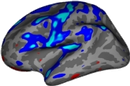
You should see something similar to this:


This figure displays the correlation between age and cortical thickness with a threshold of 4.
Notes:
The threshold is set to 4, meaning vertices with p<.0001, uncorrected, will have color. This threshold is equal to the -log(p-value). In this case, any vertex with a value under 4 will not be displayed in color, however the value will still be readable in the cursor/mouse section of freeview.
- The lower threshold sets the minimum sigificance that a voxel must meet in order to be visible. It should be set such that only likely true effects will be seen. You can kind of think of it as a filter that removes voxels where no effect is present. The upper is just used for visualization purposes. If you set it very close to the min, then all voxels will appear to be the same color. If you set it higher, then you can get some gradation due to the strength of the effect. So the min removes voxels without an effect and the max allows you to see how the strength of the effect varies across the brain.
- Blue represents a negative correlation (i.e. thickness decreases with age), red represents positive correlation (i.e. thickness increases with age).
- In this example, the sig.mgh is used as the overlay and in practice this is what is normally used. However, the pcc.mgh can also be used as the overlay if it was created in the analysis.
- Click on a point in the Precentral Gyrus. What is its value? What does it mean?
Viewing the medial surface, change the overlay threshold to something very, very low (say, .01), by clicking Configure (under the Overlay dropdown menu that says sig.mgh) and set the Min value to 0.01. Click Apply, or check the Automatically apply changes checkbox.
You should see something like this:

This figure displays the correlation between age and cortical thickness with a threshold of 0.01.
Notes:
- Almost all of the cortex now has color.
- The non-cortical areas are still blank (0) because they were excluded with --cortex in mri_glmfit above.
All the surface overlays created by mri_glmfit, not just the significance map, can also be inspected in freeview. Simply replace the path to the sig.mgh file in the command above to the surface overlay that you would like to see. For example, this will display the F ratio instead of the significance map:
freeview -f $SUBJECTS_DIR/fsaverage/surf/lh.inflated:annot=aparc.annot:annot_outline=1:overlay=lh.gender_age.glmdir/lh-Avg-thickness-age-Cor/F.mgh:overlay_threshold=20,50 -viewport 3d -layout 1
Text output and log files can be opened in any text editor.
Exercise 1
Difficulty: Intermediate
Goal: To practice setting up an analysis on subject surfaces to test an experimental hypothesis.
In the tutorial you just completed you examined the effect of age on cortical thickness, accounting for the effects of gender. In this challenge you will use the same data set to examine the effect of gender on cortical thickness, accounting for the effects of age.
Your goal is to create a new contrast file and alter the commands you used above to examine this new hypothesis. You will then open the new sig.mgh overlay which will highlight significant differences found.
Please name your new contrast file challenge-Cor.mtx Please set your GLM output directory to glm_challenge
Hints:
It will help if you start in this directory $SUBJECTS_DIR/glm and run all of your commands from there.
You will want to use mkdir glm_challenge to make the output directory, and be sure to use that directory when you run mri_glmfit
- Follow the tutorial for guidance.
- You will not need to change the FSGD file, as you are using the same groups - you don't need to change the descriptor of the groups.
You can use the command touch challenge-Cor.mtx to create a new contrast, and gedit challenge-Cor.mtx to edit it.
You will need to adjust your contrasts, consider the following snippet from the wiki page Two Groups (One Factor/Two Levels), One Covariate

- You will not need to pre-process the data, as changing the contrast doesn't have any effect on this stage.
- When you run mri_glmfit you will want to change which contrast it reads and the directory it saves to.
If you named your contrast challenge-Cor.mtx and set your output directory to glm_challenge than this command should let you examine your significance overlay.
freeview -f $SUBJECTS_DIR/fsaverage/surf/lh.inflated:overlay=glm_challenge/challenge-Cor/sig.mgh:overlay_threshold=4,5 -viewport 3d -layout 1
Want to know the answer? Highlight the text below
cd $SUBJECTS_DIR/glm |
touch challenge-Cor.mtx |
gedit challenge-Cor.mtx |
contrasts should be 1 -1 0 0 |
mri_glmfit --y lh.gender_age.thickness.10.mgh --fsgd gender_age.fsgd dods --C challenge-Cor.mtx --surf fsaverage lh --cortex --glmdir glm_challenge |
freeview -f $SUBJECTS_DIR/fsaverage/surf/lh.inflated:overlay=glm_challenge/challenge-Cor/sig.mgh:overlay_threshold=4,5 -viewport 3d -layout 1 |
You should see a few very small areas of significance, in the next tutorial you will see how running permutations affects this analysis | |
Summary
By the end of this exercise, you should know how to:
- Create a design matrix or FSGD file
- Create a contrast file
- Assemble data by running mris_preproc and mri_surf2surf
- Run a GLM analysis using mri_glmfit
- Visualize the analysis using freeview
Quiz
You can test your knowledge of this tutorial by clicking here for a quiz!