| Deletions are marked like this. | Additions are marked like this. |
| Line 156: | Line 156: |
| tkmedit fsaverage orig.mgz -aparc+aseg -overlay my-glm.wls/osgm/sig.nii.gz -fminmax 2 3 | freeview -v $SUBJECTS_DIR/fsaverage/mri/orig.mgz $SUBJECTS_DIR/fsaverage/mri/aparc+aseg.mgz:colormap=lut:opacity=0.2 my-glm.wls/osgm/sig.nii.gz:colormap=heat:heatscale=2,2,3 |
| Line 159: | Line 159: |
| * Left image is coronal slice 128 | * Left image is coronal slice 128 (make sure to click on orig so it is highlighted under the volumes tab when finding slice numbers, the slice number for the sig.nii is different) |
| Line 205: | Line 205: |
| tkmedit fsaverage orig.mgz -aparc+aseg -ov encode.merged.nii.gz -fminmax 1.3 5 -surfs | freeview -v $SUBJECTS_DIR/fsaverage/mri/orig.mgz $SUBJECTS_DIR/fsaverage/mri/aparc+aseg.mgz:colormap=lut:opacity=0.2 encode.merged.nii.gz:colormap=heat:heatscale=1.3,1.3,5 |
| Line 208: | Line 208: |
| * Left image is coronal slice 128 | * Left image is coronal slice 128 (make sure to click on the orig so it is highlighted under the volumes tab when finding slice numbers, the slice number for the sig.nii is different) |
top | previous (First Level Analysis)
Contents
1. Group Level Analysis
In general, the group analysis for fMRI is very similar to that of the structural data. There is a tutorial for this at GroupAnalysis. There are several specific differences for fMRI which are described here. In the structrual Group Analysis, you would:
- Run mris_preproc to resample each subject into the common space and then concatenate all of your subjects (one subject for each frame) into one file.
- Smoothed the data on the surface, then
- Run mri_glmfit and mri_glmfit-sim
For the function MRI group analysis you will need to:
- Concatenate individuals into one file (isxconcat-sess)
- Do not smooth (already smoothed during first-level analysis)
- Run mri_glmfit using weighted least squares (WLS)
- Correct for multiple comparisons
- Perform the above in each space (lh, rh, and mni305)
- Correct for multiple comparisons across the three spaces
- Optionally merge the three spaces into one volume space
Start the tutorial in the Project directory
setenv SUBJECTS_DIR $TUTORIAL_DATA/fsfast-tutorial.subjects
cd $TUTORIAL_DATA/fsfast-functional
2. Concatenating the Data
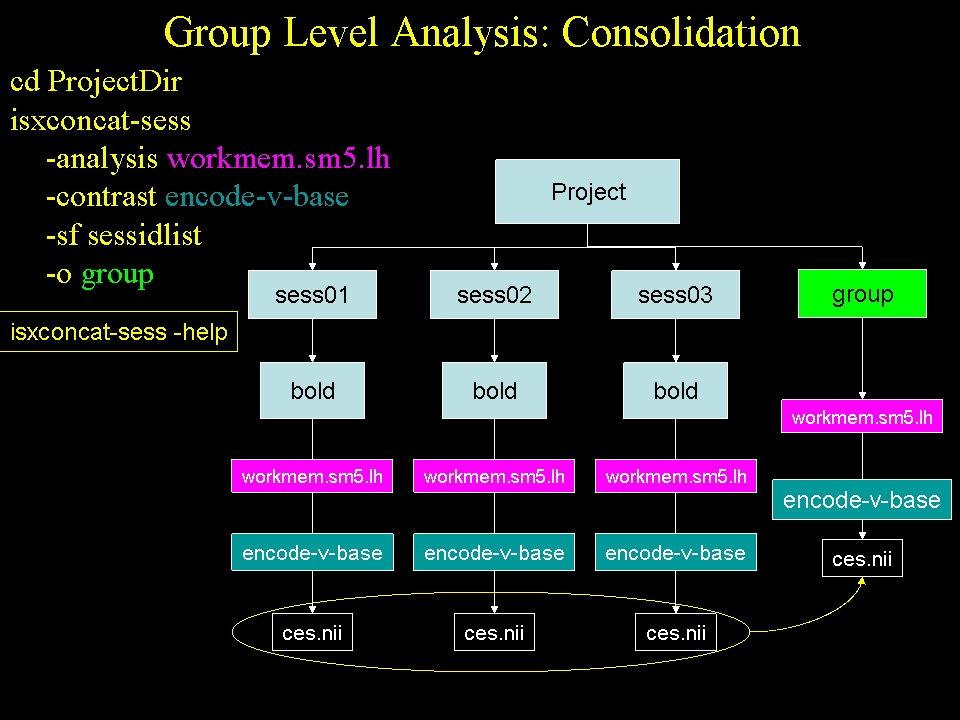
In the structural stream (see GroupAnalysis), the subject's data were concatenated into one file with mris_preproc . For the functional stream, the program is called isxconcat-sess:
isxconcat-sess -sf sessidlist -analysis workmem.sm05.lh -contrast encode-v-base -o my-group
- -sf sessidlist : use all the subjects listed in sessidlist (order is important!)
- -analysis workmem.sm05.lh : analysis from mkanalysis-sess and selxavg3-sess
- -contrast encode-v-base : contrast from mkcontrast-sess
- -o my-group : output folder is called 'my-group'
- Note: -all-contrasts can be used instead of -contrast
- Gets the contrast values (ces.nii.gz) for each subject and concatenates them into one file
- Does the same for the contrast variances (cesvar.nii.gz)
- Creates other files as well that can be used for checking for quality
 Run the concatenation for the right hemisphere and mni305 spaces
isxconcat-sess -sf sessidlist -analysis workmem.sm05.rh -contrast encode-v-base -o my-group
isxconcat-sess -sf sessidlist -analysis workmem.sm05.mni305 -contrast encode-v-base -o my-group
When this is complete, a directory called 'my-group' will be created. cd into this directory and see what's there:
cd $TUTORIAL_DATA/fsfast-functional/my-group
ls
- grouplist.txt : list of the sessions
subjectlist.txt : list of the corresponding FreeSurfer subject IDs
- sess.info.txt : other information about each session
- workmem.sm05.lh - left hemisphere analysis output folder
- workmem.sm05.rh - right hemisphere analysis output folder
- workmem.sm05.mni305 - MNI 305 analysis output folder
Go into the workmem.sm05.lh and see what's there:
cd $TUTORIAL_DATA/fsfast-functional/my-group/workmem.sm05.lh
ls
You will see several files and folders:
- analysis.info - copy of the analysis.info created by mkanalysis-sess
- meanfunc.nii.gz - a stack of the mean functional images for each session
- masks.nii.gz - a stack of the masks of all the individual subjects
- mask.nii.gz - a single mask based on the intersection of all masks
- fsnr.nii.gz - a stack of the functional SNRs for each session
- ffxdof.dat - text file with the total number of DOF summed over all sessions
- encode-v-base - folder with lower-level contrasts for the group of sessions
Each of the volumes is in the output space (lh, rh, mni305), as can be verified with mri_info. Go into the contrast folder and see what's there:
cd $TUTORIAL_DATA/fsfast-functional/group/workmem.sm05.lh/encode-v-base
ls
- Note: using 'group' instead of 'my-group'
- ces.nii.gz - stack of all the contrast values from the lower level, one for each session
- cesvar.nii.gz - stack of all the contrast variances from the lower level, one for each session
These are going to be the inputs for the group GLM analysis.
3. Run the Group GLM for the Left Hemisphere
Details on how to run the GLM are given in GroupAnalysis, including the use of FSGD files to construct complicated group-level design matrices. Here we are going to use a very simple design in which test whether the mean across the groups equals 0 (the One Sample Group Mean, or OSGM). This just requires a design matrix with a single column of all ones (created with the --osgm flag):
mri_glmfit --y ces.nii.gz \
  --wls cesvar.nii.gz \
  --osgm \
  --surface fsaverage lh \
  --glmdir my-glm.wls \
  --nii.gz
- --y ces.nii.gz : the input values to analyze
- --wls cesvar.nii.gz : variance weighting
- --osgm : use One-Sample Group Mean
- --surface fsaverage lh : indicates surface based data (not used for volume data)
- --glmdir my-glm.wls : output directory
- --nii.gz : use compressed NIFTI as output format
The one difference between this and the call in the structrual stream is the presence of the '--wls cesvar.nii.gz' option. cesvar.nii.gz is the variance of each session at each voxel. This is used to de-weight a session with high variance. This is not a true mixed effects analysis (this has been referred to as 'psuedo mixed effects'; see Thirion, 2007, Neuroimage). This step is not performed in the structural stream because we do not have variance information for each subject.
3.1. Visualize the Results of the Group GLM
tksurfer fsaverage lh inflated -aparc -overlay my-glm.wls/osgm/sig.nii.gz -fminmax 2 3
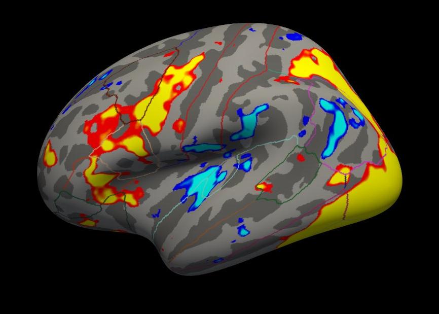
-fminmax 2 3 : threshold set to 2 (p<.01), saturation to 3 (p<.001)
- Uncorrected p-values
- Positve and negative values
3.2. Correct for Multiple Comparisons
The correction is the same as for the structural group analysis. For example, run:
mri_glmfit-sim --glmdir my-glm.wls --cache 3 pos --cwpvalthresh .0166
- --glmdir my-glm.wls : output from mri_glmfit command
- --cache 3 pos
- Use pre-cached simulation
Voxel-wise threshold of 3 (p<.001)
- Use positive contrast values
--cwpvalthresh .0166 : Cluster-wise p-value threshold. Only keep clusters that have p<.0166
Using a cluster-wise p-value threshold of p < .0166 corrects across all three spaces for p<.05 (ie, .0166 = .05/3). This corrections for a whole brain (ie, lh, rh, and subcortical) analysis. This will create several outputs, though there are three that are most important:
- cache.th30.pos.sig.cluster.summary - cluster summary table (simple ASCII text)
- cache.th30.pos.sig.cluster.nii.gz - overlay with significant clusters
- cache.th30.pos.ocn.annot - annotation of significant clusters
- Name indicates how correction was done (cache, thresh = 3, pos sign)
View the left hemisphere cache.th30.pos.sig.cluster.summary table
cat my-glm.wls/osgm/cache.th30.pos.sig.cluster.summary
View the clusters on the surface
tksurfer fsaverage lh inflated \
  -overlay my-glm.wls/osgm/cache.th30.pos.sig.cluster.nii.gz \
  -annot ./my-glm.wls/osgm/cache.th30.pos.sig.ocn.annot -fminmax 1.3 3
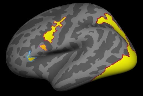
All clusters are whole-brain corrected at p<.05
- All positive because only positive was selected.
- Annotation gives cluster number
4. Right Hemisphere
Perform the same operations above for the right hemisphere (ie, go into workmem.sm05.rh):
cd $TUTORIAL_DATA/fsfast-functional/group/workmem.sm05.rh/encode-v-base
mri_glmfit --y ces.nii.gz --wls cesvar.nii.gz --osgm \
  --surface fsaverage rh --glmdir my-glm.wls --nii.gz
mri_glmfit-sim --glmdir my-glm.wls --cache 3 pos --cwpvalthresh .0166
View the right hemisphere cache.th30.pos.sig.cluster.summary table
cat my-glm.wls/osgm/cache.th30.pos.sig.cluster.summary
5. Subcortical (MNI 305 Space)
Perform the same operations above for the MNI 305 space analysis (ie, go into workmem.sm05.mni305). There are a couple of things that are different about this analysis.
cd $TUTORIAL_DATA/fsfast-functional/group/workmem.sm05.mni305/encode-v-base
ls
This directory has the same files as the surface-based results, though their dimensions are different. All the volumes here are true volumes. The mri_glmfit command is the same as for the surface-based analysis but without the (--surface fsaverage lh) part:
cd $TUTORIAL_DATA/fsfast-functional/group/workmem.sm05.mni305/encode-v-base
mri_glmfit --y ces.nii.gz --wls cesvar.nii.gz --osgm  \
  --glmdir my-glm.wls --nii.gz
freeview -v $SUBJECTS_DIR/fsaverage/mri/orig.mgz $SUBJECTS_DIR/fsaverage/mri/aparc+aseg.mgz:colormap=lut:opacity=0.2 my-glm.wls/osgm/sig.nii.gz:colormap=heat:heatscale=2,2,3
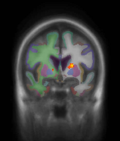
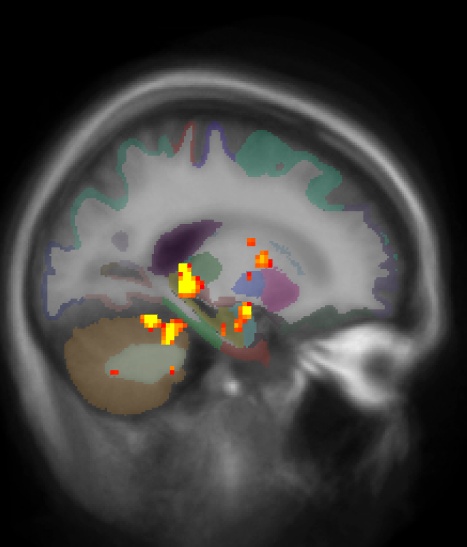
- Left image is coronal slice 128 (make sure to click on orig so it is highlighted under the volumes tab when finding slice numbers, the slice number for the sig.nii is different)
- Right image is sagittal slice 149
- No activation in cortical areas
- Positive and negative uncorrected p-values
-fminmax 2 3 : Voxel-wise threshold of 2 (p<.01), color saturation at 3 (p<.001)
To correct the subcortical analysis for multiple comparisons run:
mri_glmfit-sim --glmdir my-glm.wls --grf 3 pos --cwpvalthresh .0166
- As with the surface-based analysis, a summary file is created called grf.th3.pos.sig.cluster.summary
- Creates grf.th3.pos.sig.ocn.anat.nii.gz and grf.th3.pos.sig.ocn.lut. These are segmentations of the clusters.
View the subcortical grf.th3.pos.sig.cluster.summary table
cat my-glm.wls/osgm/grf.th3.pos.sig.cluster.summary
There are five clusters for the subcortical analysis. View the corrected results in the volume:
tkmedit fsaverage orig.mgz \
  -ov my-glm.wls/osgm/grf.th3.pos.sig.cluster.nii.gz \
  -seg ./my-glm.wls/osgm/grf.th3.pos.sig.ocn.anat.nii.gz  \
       ./my-glm.wls/osgm/grf.th3.pos.sig.ocn.lut \
-fminmax 1.3 5- Only positive values
- p-values are p-values for cluster
Set threshold to 1.3 (p<.05)
6. Merging the Results
These three tables give you the clusters across the whole brain for Left Hemisphere Right Hemisphere Subcortical
cd $TUTORIAL_DATA/fsfast-functional/group
cat workmem.sm05.lh/encode-v-base/my-glm.wls/osgm/cache.th30.pos.sig.cluster.summary
cat workmem.sm05.rh/encode-v-base/my-glm.wls/osgm/cache.th30.pos.sig.cluster.summary
cat workmem.sm05.mni305/encode-v-base/my-glm.wls/osgm/grf.th3.pos.sig.cluster.summary
Merge the corrected results into a single volume for visualization
vlrmerge --o encode.merged.nii.gz \
  --lh workmem.sm05.lh/encode-v-base/my-glm.wls/osgm/cache.th30.pos.sig.cluster.nii.gz \
  --rh workmem.sm05.rh/encode-v-base/my-glm.wls/osgm/cache.th30.pos.sig.cluster.nii.gz \
  --vol workmem.sm05.mni305/encode-v-base/my-glm.wls/osgm/grf.th3.pos.sig.cluster.nii.gz \
  --scm workmem.sm05.mni305/subcort.mask.nii.gz
Creates encode.merged.nii.gz by mapping the left and right hemispheres to the volume and merging with the subcotical results. View the merged volume
freeview -v $SUBJECTS_DIR/fsaverage/mri/orig.mgz $SUBJECTS_DIR/fsaverage/mri/aparc+aseg.mgz:colormap=lut:opacity=0.2 encode.merged.nii.gz:colormap=heat:heatscale=1.3,1.3,5
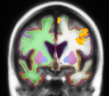
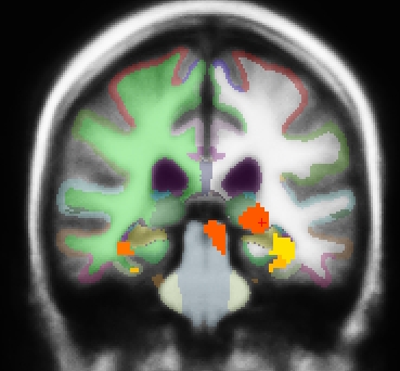
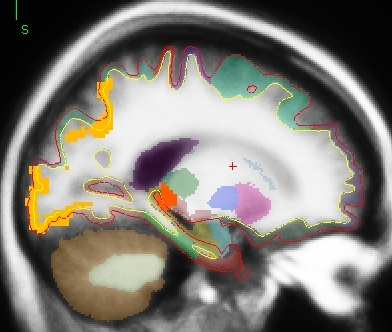
- Left image is coronal slice 128 (make sure to click on the orig so it is highlighted under the volumes tab when finding slice numbers, the slice number for the sig.nii is different)
- Middle image is coronal slice 95
- Right image is sagittal slice 149
- Color indicates cluster p-value.
- All positive because only positive was selected.
- Cortical activation comes from the cortical analysis
- Subcortical activation comes from the subcortical analysis
All activation in this image has been corrected for whole-brain multiple comparisons a p<.05.
